predictcomp
- predictcomp(objname='', standard='Butler-JPL-Horizons 2010', epoch='', minfreq='', maxfreq='', nfreqs=2, prefix='', antennalist='', showplot=False, savefig='', symb='.', include0amp=False, include0bl=False, blunit='', showbl0flux=False)[source]
Make a component list for a known calibrator
[Description] [Examples] [Development] [Details]
- Parameters
objname (string=’’) - Object name
standard (string=’Butler-JPL-Horizons 2010’) - Flux density standard
epoch (string=’’) - Epoch
minfreq (string=’’) - Minimum frequency
maxfreq (string=’’) - Maximum frequency
nfreqs (int=2) - Number of frequencies
prefix (path=’’) - Prefix for the component list directory name.
antennalist (string=’’) - Plot for this configuration
antennalist != ''
showplot (bool=False) - Plot S vs |u| to the screen?
savefig (string=’’) - Save a plot of S vs |u| to this filename
symb (string=’.’) - A matplotlib plot symbol code
include0amp (bool=False) - Force the amplitude axis to start at 0?
include0bl (bool=False) - Force the baseline axis to start at 0?
blunit (string=’’) - unit of the baseline axis
showbl0flux (bool=False) - Print the zero baseline flux ?
symb (string=’.’) - A matplotlib plot symbol code
- Returns
components (dict) - list of components and additional information including object name, standard, epoch, frequencies and antennas configuration file
- Description
This task makes a flux model as a component list from one of the flux calibrator standards used by the setjy task. It also returns a Python dictionary of the predicted model and optionally plots the predicted visibility amplitudes versus uv-distance when the array configuration information is specified. It uses the same common prediction code as setjy but without the need for the actual visibility data. This task is useful for cross checking what setjy would set for model visilibilities or for finding a predicted flux density for a calibrator at a particular epoch, especially when the flux calibrator is a Solar System object.
The following are the main keys of the returned dictionary (or False on error):
‘antennalist’ - array configuration file
‘savedfig’ - output file name for a plot
‘spectrum’ - frequency setup information
‘clist’ - output component list name
‘riseset’ - times of rise and set of the object
‘standard’ - flux standard used
‘shape’ - model shape and position of the object
‘epoch’ - epoch used
‘objname’ - object name
‘freqs (GHz)’ - frequencies
‘amps’ - list of predicted visibility amplitudes
‘baselines’ - list of baselines
‘blunit’ - unit
‘azel’ - AZ-El direction
Parameter descriptions
objname
The object name as recognized by setjy. If the object specified is not visible from the specified telescope, an error will be thrown to this effect.
standard
Sets the flux density model standard from setjy, namely Perley-Taylor 99, Baars, Perley 90, Perley-Taylor 95, Butler-JPL-Horizons 2010, Butler-JPL-Horizons 2012.
epoch
Sets the time that predictcomp uses, which is only relevant for Solar Object standards, using a standard CASA date/time format (e.g., ‘2018-12-31/5:34:12’).
minfreq
Sets the minimum predicted frequency of the model. Units must be given. Examples: minfreq=’230GHz’
maxfreq
Sets the maximum predicted frequency of the model. Units must be given. Examples: maxfreq=’265GHz’
nfreqs
Sets the frequency interval for the predicted visibilities. Examples: minfreq=’230GHz’ maxfreqs=’265GHz’ nfreqs=5, the predicted visibilities will be determined for frequencies of equal interval determined by the equation \((maxfreqs - minfreqs) / nfreqs\) (in this case, for frequencies 230, 239, 248, 256, and 265 GHz).
prefix
The component list will be saved to ‘<prefix> + <objname>_spw0_<minfreq><epoch>.cl’. If a component list of the same name already exists, predictcomp will remove the previous version. Default: ‘ ‘ which will create the component list name sans the prefix. Examples: prefix=’Bands3to7_’, which could produce ‘Bands3to7_Uranus_spw0_100GHz55877d.cl’ (depending on the other parameters).
antennalist
When antennalist is given a valid array configuration file, the task predicts and plots (if set) the visibility amplitudes for the array configuration. The search path is: .:casa[‘dirs’][‘data’] + ‘/alma/simmos/’. Default: ‘’, None just makes a component list. Examples: antennalist=’alma.cycle0.extended.cfg’
antennalist expandable parameters
showplot
Whether or not to show a plot of the visibility amplitudes vs. uv distance on the screen.
savefig
Filename for saving a plot of the amplitude vs. uv distances.
symb
One of matplotlib’s codes for plot symbols: .:,o^v<>s+xDd234hH|_. Default: ‘.’
include0amp
Force the amplitude axis to start at 0. Default: False
include0bl
Force the baseline axis to start at 0. Default: False
blunit
Unit of the baseline axis (’’ or ‘klambda’). Default: ‘ ‘ = use a unit in the data
showbl0flux
Print the zero baseline flux. Default: False
- Examples
CASA <1>: predictcomp(objname="Uranus", standard="Butler-JPL-Horizons 2012",
                      epoch="2018/06/01/12:00", minfreq="100GHz", maxfreq="120GHz", nfreqs=2)
Will create a model of Uranus in component list, Uranus_spw0_100.000GHz_58270.5d.cl, on a disk using Butler-JPL-Horizons 2012.
Out[1]:
{'antennalist': '',
 'clist': 'Uranus_spw0_100.000GHz_58270.5d.cl',
 'epoch': {'m0': {'unit': 'd', 'value': 58270.5},
           'refer': 'UTC',
           'type': 'epoch'},
 'freqs (GHz)': array([ 100.,  120.]),
 'objname': 'Uranus',
 'savedfig': None,
 'shape': {'direction': {'error': {'latitude': {'unit': 'rad', 'value': 0.0},
                                   'longitude': {'unit': 'rad', 'value': 0.0}},
                         'm0': {'unit': 'rad', 'value': 0.5004200115883465},
                         'm1': {'unit': 'rad', 'value': 0.195254121510741},
                         'refer': 'J2000',
                         'type': 'direction'},
           'majoraxis': {'unit': 'arcmin', 'value': 0.056882862988833334},
           'majoraxiserror': {'unit': 'rad', 'value': 0.0},
           'minoraxis': {'unit': 'arcmin', 'value': 0.05558989939983334},
           'minoraxiserror': {'unit': 'rad', 'value': 0.0},
           'positionangle': {'unit': 'deg', 'value': 0.0721226031886111},
           'positionangleerror': {'unit': 'rad', 'value': 0.0},
           'type': 'Disk'},
 'spectrum': {'freqRef': {'m0': {'unit': 'Hz', 'value': 0.0},
                          'refer': 'TOPO',
                          'type': 'frequency'},
              'frequency': {'m0': {'unit': 'GHz', 'value': 100.0},
                            'refer': 'TOPO',
                            'type': 'frequency'},
              'ival': array([  8.04191982,  10.59860209]),
              'maxFreq': 120000000000.0,
              'minFreq': 100000000000.0,
              'qval': array([ 0.,  0.]),
              'referenceFreq': 100000000000.0,
              'tabFreqVal': array([  1.00000000e+11,   1.20000000e+11]),
              'type': 'Tabular Spectrum',
              'uval': array([ 0.,  0.]),
              'vval': array([ 0.,  0.])},
 'standard': 'Butler-JPL-Horizons 2012'}
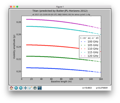
To plot Titan’s predicted model on 2017/10/15/00:00 for alma.cycle5.1 array configuration,
CASA <4>: predictcomp(objname="Titan",standard="Butler-JPL-Horizons 2012",
                      epoch="2017/10/15/00:00",minfreq="100GHz",maxfreq="120GHz",
                      nfreqs=5,antennalist="alma.cycle5.1.cfg",showplot=True,
                      savefig="visplot.png")
Will return a dictoionary and show a plot along with a model in a component list, Titan_spw0_100.000GHz_58041.0d.cl on disk,
Out[4]: {'amps': array([[ 0.20578021,  0.20568487,  0.20565192, ...,
                          0.20564561,  0.20559302,  0.20549726],
                        [ 0.22465639,  0.22454165,  0.224502  , ...,
                          0.22449438,  0.2244311 ,  0.22431585],
                        [ 0.24305519,  0.24291895,  0.24287187, ...,
                          0.24286284,  0.2427877 ,  0.24265087],
                        [ 0.27325127,  0.27308387,  0.27302599, ...,
                          0.2730149 ,  0.27292258,  0.27275446],
                        [ 0.28463319,  0.28444329,  0.28437769, ...,
                          0.28436509,  0.28426039,  0.28406972]]),
'antennalist': '/home/casa/data/distro/alma/simmos/alma.cycle5.1.cfg',
'azel': {'m0': {'unit': 'rad', 'value': -1.7483672182501997},
         'm1': {'unit': 'rad', 'value': 0.7161180761232981},
         'refer': 'AZEL',
         'type': 'direction'},
'baselines': array([  10.96451651,   20.85185229, 23.31405119,   54.00490666,
                      38.87662356,   33.66407931,   35.35062247, 48.63818994,
                      57.99592862,   56.0237924 ,   23.94816258, 56.38958284,
                      77.29513965,   30.66467013,   13.2990365 , 11.29543388,
          ...

                      14.92214009,   12.19798989,   35.79226375, 29.69284989,
                      23.75722946,   27.16544565,   32.46739665]),
'blunit': 'm',
'clist': 'Titan_spw0_100.000GHz_58041.0d.cl',
'epoch': {'m0': {'unit': 'd', 'value': 58041.0},
          'refer': 'UTC',
          'type': 'epoch'},
'freqs (GHz)': array([ 100.,  105.,  110.,  115.,  120.]),
'objname': 'Titan',
'riseset': {'NOTE': 'APPROXIMATE.  The times do not account for the apparent motion of Titan.',
'rise': {'last': {'m0': {'unit': 'd', 'value': 64771.451977904355},
                  'refer': 'LAST',
                  'type': 'epoch'},
         'str': '2017-10-14/13:48:40 UTC (MJD 58040.58)',
         'utc': {'m0': {'unit': 'd', 'value': 58040.575471333046},
                 'refer': 'UTC',
                 'type': 'epoch'}},
'set': {'last': {'m0': {'unit': 'd', 'value': 64772.00711916989},
                 'refer': 'LAST',
                 'type': 'epoch'},
        'str': '2017-10-15/03:05:53 UTC (MJD 58041.13)',
        'utc': {'m0': {'unit': 'd', 'value': 58041.129096842145},
        'refer': 'UTC',
        'type': 'epoch'}}},
'savedfig': 'visplot.png',
'shape': {'direction': {'error': {'latitude': {'unit': 'rad', 'value': 0.0},
                                  'longitude': {'unit': 'rad', 'value': 0.0}},
                                  'm0': {'unit': 'rad', 'value': -1.703860578032794},
                                  'm1': {'unit': 'rad', 'value': -0.38749817506070633},
                                  'refer': 'J2000',
                                  'type': 'direction'},
                        'majoraxis': {'unit': 'arcmin', 'value': 0.011260686213666667},
                        'majoraxiserror': {'unit': 'rad', 'value': 0.0},
                        'minoraxis': {'unit': 'arcmin', 'value': 0.011260686213666667},
                        'minoraxiserror': {'unit': 'rad', 'value': 0.0},
                        'positionangle': {'unit': 'deg', 'value': 0.0013638055555555554},
                        'positionangleerror': {'unit': 'rad', 'value': 0.0},
                        'type': 'Disk'},
          'spectrum': {'bl0flux': {'unit': 'Jy', 'value': 0.20581664144992828},
          'freqRef': {'m0': {'unit': 'Hz', 'value': 0.0},
          'refer': 'TOPO',
          'type': 'frequency'},
'frequency': {'m0': {'unit': 'GHz', 'value': 100.0},
              'refer': 'TOPO',
              'type': 'frequency'},
'ival': array([ 0.20581664,  0.22470025,  0.24310728,  0.27331526,  0.28470576]),
'maxFreq': 120000000000.0,
'minFreq': 100000000000.0,
'qval': array([ 0.,  0.,  0.,  0.,  0.]),
'referenceFreq': 100000000000.0,
'tabFreqVal': array([  1.00000000e+11,   1.05000000e+11,  1.10000000e+11,  1.15000000e+11,   1.20000000e+11]),
'type': 'Tabular Spectrum',
'uval': array([ 0.,  0.,  0.,  0.,  0.]),
'vval': array([ 0.,  0.,  0.,  0.,  0.])},
'standard': 'Butler-JPL-Horizons 2012'}
Type
Figure
ID
1
Caption
Predicted visibilities plot for Titan.
- Development
No additional development details
- Parameter Details
Detailed descriptions of each function parameter
objname (string='')- Object namestandard (string='Butler-JPL-Horizons 2010')- Flux density standardepoch (string='')- Epochminfreq (string='')- Minimum frequencymaxfreq (string='')- Maximum frequencynfreqs (int=2)- Number of frequenciesprefix (path='')- Prefix for the component list directory name.antennalist (string='')- Plot for this configurationshowplot (bool=False)- Plot S vs |u| to the screen?savefig (string='')- Save a plot of S vs |u| to this filenamesymb (string='.')- A matplotlib plot symbol codeinclude0amp (bool=False)- Force the amplitude axis to start at 0?include0bl (bool=False)- Force the baseline axis to start at 0?blunit (string='')- unit of the baseline axisshowbl0flux (bool=False)- Print the zero baseline flux ?