Open in Colab: https://colab.research.google.com/github/casangi/casadocs/blob/master/docs/notebooks/memo-series.ipynb
CASA Memos
CASA Memo Series
CASA Memo 1: MeasurementSet Definition version 2.0 - A.J. Kemball & M.H. Wieringa, v. 01/2000
CASA Memo 2: Convention for UVW calculations in CASA - U. Rau, v. 02/2013
CASA Memo 3: MeasurementSet Selection Syntax - S. Bhatnagar, v. 06/2015
CASA Memo 4: CASA Imager Paralellization: Measurement and Analysis of Runtime Performance for Continuum Imaging - S. Bhatnagar & CASA HPC team, v. 03/2016
CASA Memo 5: CASA Performance on Lustre: serial vs parallel and comparison with AIPS - B. Emonts, v. 06/2018
CASA Memo 6: User Survey and Helpdesk Statistics 2018 - B. Emonts, v. 11/2018
CASA Memo 7: ALMA Mosaicing Imaging Issues Prior to Cycle 6 - North American ALMA Science Center (NAASC) Software Support Team, v. 09/2018. Copy of NAASC Memo 117 (credit: NAASC).
CASA Memo 8: Non-Amnesic CLEAN: A boxless/maskless CLEAN style deconvolution algorithm - K. Golap, v. 12/2015
CASA Memo 9: Improvements to Multi-Scale CLEAN and Multi-Term Multi-Frequency CLEAN - J.-W. Steeb & U. Rau, v. 07/2019
CASA Memo 10: Restoring/Common Beam and Flux Scaling in tclean - J.-W. Steeb & U. Rau, v. 08/2019
CASA Memo 11: Heterogeneous Pointing Corrections in AW-Projection - P. Jagannathan & S. Bhatnagar 10/2019
CASA Memo 12: The Fringefit Task in CASA - D. Small & G. Moellenbrock 08/2022
CASA Memo 13: Cube Parallelization with CASA - S.Sekhar, U.Rau & R.Xue 08/2024
CASAcore Memos
CASA’s underlying structure is based on casacore. The CASAcore Notes describe some of the most fundamental properties, such as on the table system, data selection syntax, and data model definitions.
AIPS++ Memos
The origin of CASA lies in the AIPS++ project [1,2], which was started in 1992 as the successor of the Astronomical Information Processing System (AIPS) software package [3]. In 2004, the AIPS++ code was re-organized and migrated to CASA. The AIPS++ memos can be found here.
Bibliography
Glendenning, B. E. 1996, Astronomical Data Analysis Software and Systems V, Vol. 101 (San Francisco, CA: ASP), 271
McMullin, J. P., Shiebel, D. R., Young, W., & Debonis, D. 2006, in ASP Conf. Ser. 351, Astronomical Data Analysis Software and Systems XV (San Francisco, CA: ASP), 319
Greisen, E. W. 2003, Information Handling in Astronomy—Historical Vistas, Vol. 285 (Dordrecht: Kluwer), 109
CASA Knowledgebase
The CASA Knowledgebase pages provide bits of wisdom on CASA that should be preserved, and that may be of use to expert users.
Installation
Knowledgebase items related to installing CASA on various Operating Systems.
Pre-requisites Libraries
CASA requires certain libraries be installed in the users operating system. Some may already be present by default. In case they are not, the following list should be checked before using CASA or if errors are encountered at runtime.
Commands and package names are for Red Hat Linux, but equivalents can be found for other Linux distributions.
FUSE
The AppImage software is used to package the GUIs that are part of CASA. Users need to have the FUSE software installed, so these applications can be mounted and CASA can be run in its entirety.
OS Libraries
A system administrator may be required to install OS libraries. For example, for RHEL8 the following OS libraries should be installed:
$: sudo yum install ImageMagick*$: sudo yum install xorg-x11-server-Xvfb$: sudo yum install compat-libgfortran-48$: sudo yum install libnsl$: sudo yum install libcanberra-gtk2
ImageMagick can be obtained from EPEL 8: https://dl.fedoraproject.org/pub/epel/8/Everything/x86_64/Packages/i/. To add Epel via subscription manager (from RHEL docs):
$: subscription-manager repos --enable codeready-builder-for-rhel-8-$(arch)-rpms$: dnf install https://dl.fedoraproject.org/pub/epel/epel-release-latest-8.noarch.rpm
Other packages that may need to be installed are:
$: sudo yum install fuse$: sudo yum install perl
Modular CASA
For modular CASA, one must supply their own Python environment. There are many, including ipython and Jupyter, here is a basic example:
$: sudo yum install python36-develorpython38-devel
MPI (parallel processing)
When using the casampi package from modular CASA, additional MPI libraries are needed:
$: sudo yum install openmpi-devel$: sudo yum install mpich-develUser installs mpi4py with:
-    ```$: env MPICC=/usr/lib64/openmpi/bin/mpicc python -m pip install mpi4py --no-cache-dir```
-    Ensure mpirun is found: ```which mpirun```
-    If not, try full path: ```export PATH=/usr/lib64/openmpi/bin/mpirun\$PATH```
Pipeline
For running the pipeline within CASA, poppler-utils may also have to be installed.
NRAO internal
Alternative method for NRAO systems only:
contact the helpdesk to install casa-toolset-3 (which contains the previous libraries)
the run
export PATH=/opt/casa/03/bin:\$PATH
Additional Pre-requisites Mac OS
In addition to the general pre-requisites for running CASA, users should be aware of the following pre-requisites for Mac OS.
CASA Viewer
The CASA Viewer is no longer packaged with the monolithic CASA for Mac OS.
Using the modular CASA Viewer with Mac OS requires a special setup step. Download and expand the pgplot installation files on your machine. Then set the following environment variables from a terminal:
export PGPLOT_DIR=<download location>/pgplot
export PGPLOT_FONT=<download location>/pgplot/grfont
Installing mutiple Python versions on Mac OS 11
One solution for handling multiple Python installations across versions (e.g. Python 3.6 and 3.8) is to use pyenv.
Pyenv can be installed on Mac OS 11 a number of ways, but perhaps the simplest is to use homebrew:
brew install pyenv
Installation of a given version of Python via pyenv is normally a single simple command such as:
pyenv install 3.8.0
which can be repeated for each version of Python desired.
For Mac OS 11, however, there is currently a known issue preventing this simple command from working. As a workaround, the following command has worked in testing on Mac OS 11 with an Intel x86 64 bit architecture. See the github issue, however, for the most up to date information on the bug.
CFLAGS="-I$(brew --prefix openssl)/include -I$(brew --prefix bzip2)/include -I$(brew --prefix readline)/include -I$(xcrun --show-sdk-path)/usr/include"
LDFLAGS="-L$(brew --prefix openssl)/lib -L$(brew --prefix readline)/lib -L$(brew --prefix zlib)/lib -L$(brew --prefix bzip2)/lib"
arch -x86_64 pyenv install --patch 3.8.0 < <(curl -sSL https://github.com/python/cpython/commit/8ea6353.patch\?full_index\=1)
In this example, 3.8.0 may be replaced by the desired installation version of Python.
Finally, the .zshrc file (or similar configuration file for your desired terminal) should be modified to include the following:
PYENV_ROOT=/Users/username/.pyenv
export PATH="$PYENV_ROOT/bin:$PATH"
export PATH="$PYENV_ROOT/shims:$PATH"
eval "$(pyenv init -)"
With this complete, the Python version can be switched by setting the local or global Python using pyenv, and then restarting the terminal. Modular CASA can then be installed within a virtual environment following the instructions on the CASA Installation page.
pyenv local 3.8.0
pyenv global 3.8.0
Installing CASA on FIPS-enabled machines
Disclaimer: the information in this Section is provided by users and does not reflect official CASA recommendations. The information should be used at your own risk.
For machines that are configured to Federal Information Processing Standards (FIPS), the monolithic CASA version may fail to start. The reason is that CASA invokes its own crypto and ssl libraries, whereas FIPS compliance requires use of the system-controlled libraries. These CASA-invoked libraries are essential for CASA to work on Ubuntu machines, and it is therefore unlikely that this will change in the foreseeable future.
Attached is a PDF with workaround solution for installing CASA on FIPS-enabled machines. This workaround solution is kindly provided by S. White and J. Newlander at the Air Force Research Lab.
User tips on installing CASA on unsupported OSs
This document provide tips from users on how to install CASA on unsupported operating systems, like LINUX Debian and Fedora.
Disclaimer: the information in this document is provided by users and not verified by the CASA team. The information does not reflect official CASA recommendations and should be used at your own risk.
CASA officially supports certain versions of LINUX Redhat and Mac OSX. See the CASA Download page for more information.
We realize that many users wish to try and run CASA on different operating systems. Below are some tips from the user community on installing CASA on unsupported platforms. CASA will not run on Windows.
Ubuntu or Debian - Please see the following PDF: Installing CASA on Unbuntu or Debian
Fedora - Fedora 32 may cause CASA to crash on startup with the error “code for hash md5 was not found”. This is caused by changes to libssl.so in the compat-openssl10 package, which prevents the CASA supplied version of this library from loading. An easy fix is to replace the CASA version of libssl.so.10 with the OS version in /lib64 (i.e., libssl.so.1.0.2o).
Data Processing
General Knowledgebase items on data processing.
Correcting bad common beam
This script re-calculates the common beam by discarding certain channels where the point-spread-function (PSF) or ‘beam’ deviates substantially from those of the other channels.
It can happen that an MS contains one or more channels for which the point-spread-function (PSF) or ‘beam’ deviates a lot from those of the other channels. This can be the result of substantial flagging, missing data, or other factors. When making a data cube with restoringbeam=’common’, these “outlier” channels can create a common beam that does not reflect the beam for the bulk of the channels.
This example_robust_common_beam.py script will correct the common beam by detecting and/or flagging outliers channels in the calculation of the common beam. The outlier channels are identified as those channels for which the area of those beams deviate from the median beam by a user-specified factor in computation of the median area beam. The script will do the following:
Run tclean with niter=0
Detect/flag outliers in chan beams
Use the remaining beams with ia.commonbeam() to get a new commonbeam
Specify this explicitly to tclean in the subsequent niter>0 run.
The attach script primarily demonstrates the solution of iter0 -> calc_good_beam -> specify_restoringbeam_in_iter1 along with tclean. If the new commonbeam is not larger than all the bad beams, then the iter0 tclean run’s restoration step will throw warnings for all channels that cannot be convolved to the new common beam.
The functionality provided by this script is not yet implemented in the commonbeam method of the image analysis tool (ia.commonbeam).
Please note that the script is based on an ALMA test-data that was used for characterizing the problem in pipeline processing at the NAASC (JIRA ticket PIPE-375). Parameters have to be adjusted for each use case, including heuristics to detect outlier channels and what to substitute the ‘bad’ beams with.
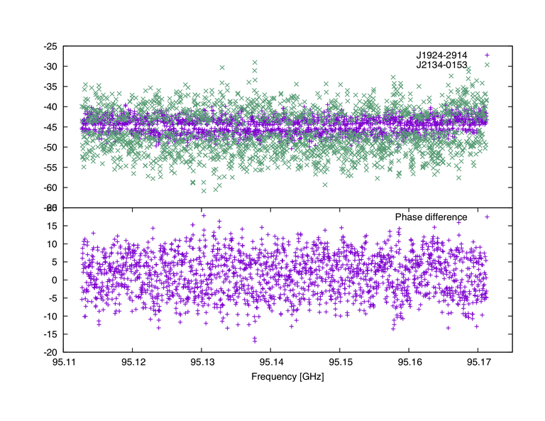
ALMA polarization: XY-phase solver avoids +-45 deg solution
The XY-phase calibration obtained with CASA task gaical (gaintype=’XYf+QU’) avoids to output +/- 45 degree solutions. This is a subtle consequence of the algorithm used to solve for the cross-hand phase, and should be harmless for the calibration of ALMA full-polarization data.
When using the task gaincal with parameter gaintype=’XYf+QU’, the solution to solve is a fit for a slope in 2D data (imag vs. real) from data that has noise is both dimensions. In such cases, it is always better to fit a shallow (not steep) slope, so if the slope (for imag vs. real) comes out >1.0, it flips the axes (to real vs. imag) and re-fits it (and inverts the resulting value to account for the swap). This minimizes the effect of the real axis noise on the slope calculation. This yields far more accurate solutions when the nominal slope is very large (>>1.0, e.g., the data nearly parallel to the imag axis == cross-hand phase approaching +/-90 deg).
The case of slope = 1.0 (which is cross-hand phase of 45 deg) corresponds to the slope at which to pivot the axis swap decision. When plotting the cross-hand phase solutions, a gap appears at +-45 deg (see figure). This gap is a property of the typical spacings between values in the statistical distribution of slope values. I.e., for a sample of N points filling a distribution with a finite width, there is a characteristic minimum spacing between values that is some small fraction of the width of the distribution. Of course, smaller spacings are not forbidden, but they are rare. The axis swap reveals this property since all of the (nominal) slopes that are >1.0 (cross-hand phases >45.0 deg) are fit with swapped data and yield the inverse slope (<1.0), and than inverted to be >1.0 again. The typical slopes mostly do not get arbitrarily close to exactly 1.0, so the gap appears. This is essentially an extension of the fact that (for any slope), the precise exact value need not be realized in any instance in a sample of solutions for it. E.g., in a sample of N gaussian-distributed values centered on some specific value the likelihood of any sample having that precise central value is vanishingly small.
The gap should become smaller when either the noise decreases, or the number of channels (for the same noise) increases.
This feature should be harmless for the calibration of ALMA full-polarization data.
Wideband Mosaic Imaging and Pointing Corrections for the VLA Sky Survey
This Knowledgebase article describes testing results for wideband mosaic imaging and pointing corrections for VLASS.
The Very Large Array Sky Survey (VLASS) critically depends on accurate wideband mosaicing algorithms for its single epoch imaging and ultimately cumulative imaging. To a large degree, VLASS requirements have driven CASA’s development of the AW-projection and related algorithms for widefield and wideband imaging in CASA. This Knowledgebase article provides complementary reports on the testing of Wideband Mosaic Imaging and Pointing Corrections for VLASS.
Calculation of Weights for Data with Varying Integration Time
Knowledgebase Article: Calculation of Weights for Data with Varying Integration Time
George Moellenbrock Original 18 Dec 2018, latest edited version 04 Nov 2019
When the nominal weights are expected to be uniform (because integration time, channel bandwidth, effective Tsys, collecting area, etc. are all uniform, or the visibilities are normalized), extracting weight information from the apparent statistics of otherwise stable visibility measurements is a simple matter of calculating the apparent simple variance in the visibility real and imaginary parts over a sufficient local sample of values. The real and imaginary part variances should be approximately equal, and the inverse of their mean is the correct weight to assign to each of the visibility values within the sample. Here, “stable visibility” means no systematic variation of amplitude or phase within the local sample. Noise-dominated visibilities are ideal; otherwise, well-calibrated data with no true visibility variation are desirable. These conditions are also needed for the more general case described below.
When the integration time (aka “exposure”) varies within the local sample (such as can be generated by averaging of the data post-correlation, where the number of samples per averaging bin may vary, especially at the end of scans), we expect the correct variance for each visibility to be inversely proportional to the net integration time, and this complicates the calculation. It is necessary to determine a weighted variance per unit inverse integration time, wherein the sample weights for the variance calculation are the per-visibility integration times, \(e_i\). If the only reason the underlying variance differs among samples is the variable integration time, then a uniform normalized variance estimate of the whole sample may be obtained by scaling the residual data per sampleby the square root of their (known) integration times. Here, residual data means any underlying visibility signal—presumably the average of the visibility samples, using nominal (proportional to integration time, etc.) weights—has been subtracted. The simple variance of thisrescaled sample is, in effect, the variance per unit inverseintegration time.
For visibilities \(V_i\), with integration times \(e_i\):
\(<\)var\(_{norm}\)\(>\) = Sum (\(e_i\) (\(V_i\) - \(<\)\(V\)\(>\))\(^2\)/\(N\) [1]
where \(<\)\(V\)\(>\) = Sum(\(w_i\)\(V_i\))/Sum(\(w_i\)) [1a]
and \(w_i\) are the nominal data weights presumably proportional tointegration time and other relevant factors. In practice, we could probably just use \(w_i\) = \(e_i\) in equation [1a] since all of the other relevant factors witin \(w_i\) are assumed constant within the sample. Note that the units of \(<\)var\(_{norm}\)\(>\) are in squared visibility amplitude (\({\rm Jy}^{2}\), presumably) times seconds. Note also that \(<\)var\(_{norm}\)\(>\) is essentially the simple variance of the ensemble \(\sqrt{(e_i)}\).d\(V_i\) (where d\(V_i\) is (\(V_i\)-\(<\)\(V\)\(>\))), i.e., of the residual visibilities scaled so that their noise is independent of integration time.
The normalized weight-per-unit-integration time is thus the inverse of \(<\)var\(_{norm}\)\(>\):
\(W_{norm}\) = 1/\(<\)var\(_{norm}\)\(>\) [2]
and per-datum revised weights may be calculated as:
\(W_i\) = \(W_{norm}\) * \(e_i\) [3]
Another way of arriving at this result is to calculate a weighted variance:
\(<\)var\(>\) = Sum(\(e_i\) (\(V_i\) - \(<\)\(V\)\(>\))\(^2\)) / Sum(\(e_i\)) [4]
which corresponds to the (simple) mean exposure time, which is:
\(<\)\(e\)\(>\) = Sum(\(e_i\)) / N [5]
The product of these yields \(<\)var\(_{norm}\)\(>\), as above in [1]:
\(<\)var\(_{norm}\)> = \(<\)var\(>\)\(<\)\(e\)\(>\) [6]
and \(W_{norm}\) may be formed and applied as in [2] and [3] above.
This calculation should be done for both real and imaginary parts ofthe visibility sample and averaged, or for both parts jointly, and [3] used to form the revised weights.
NB: In calculating sample variance, it is generally customary to acknowledge the loss of one degree of freedom due to use of the meanvisibility, \(<\)\(V\)\(>\) in the calculation. Essentially, \(<\)\(V\)\(>\) will have a finite error that tends to bias the resulting variance downward. For simple variance calculations, a factor N/(N-1) is applied to the variance calculation to unbias it, and this factor can be significant for modest N. Since a non-trivially weighted mean is used in the above (otherwise simple, non-weighted) variance calculation (eqn [1]), it may be appropriate to consider a more carefully weighted calculationfor the N/(N-1) factor. The required factor is:
D = 1 - ( Sum(\(w_i\)\(^2\)) / Sum(\(w_i\))\(^2\) ) [9]
where \(w_i\) are the a priori nominal weights used in [1a] above. This factor can be shown to equal (N-1)/N and so should be divided into the \(<\)var\(_{norm}\)\(>\) result.
However, since the nominal error in the variance (and thus the weights) will be <10% (an accuracy we are unlikely to achieve ingeneral anyway) for N>10, and will be uniform over many sample groups in the overall statwt execution, we assume that it is adequate to use thesimpler N/(N-1) factor, or omit it entirely.
Bug affecting polarization visibility data in concatenated data
Knowledgebase Article: characterization of a bug that affected polarization visibility data in concatenated data in CASA versions up to 5.6.
George Moellenbrock Original 17 Apr 2020, latest edited version 12 May 2020
CASA 5.7/6.1 fixed a bug in concat and importfitsidi that affected polarization visibility data in concatenated MSs. The problem that occurs in CASA versions earlier than 5.7/6.1 is that the cross-hands may be spuriously mis-ordered on a subset of baselines in the concatenated MS.This Knowledgebase Article describes the main effects that this bug has on concat’d data in general, and in particular on the processing of ALMA and VLA data with CASA up to and including version 5.6.A careful analysis has revealed the following effects in concat’d MSs in CASA versions prior to 5.7/6.1:
In general, visibility data cross-hands may be spuriously swapped on some baselines in concat’d data when the antenna lists in the input MSs are partially different. The concat task adopts the first (in time order) MS’s antenna list for the output MS, and appends unique antennas from later MS(s), typically with larger indices than in their original MSs. Depending on the original antenna indexing, baselines between these additional antennas and antennas that did occur in the first MS may sometimes require conjugation (reversal of the order of antennas in the baseline) to maintain internal indexing consistency within the output MS (for all baselines in an MS, the first antenna must have an index which is lower than (or same as) the index of the second antenna). When baselines are conjugated in this way, the sign of the phase of each correlation and the UVWs must be reversed, and the cross-hands swapped (RL or XY will become LR or YX, respectively, and vice-versa). Prior to CASA 5.7/6.1, the sign reversals were correct, but the cross-hand swap was spuriously omitted. For successfully calibrated data (i.e., calibrated prior to running concat), this means that the sign of the imaginary part of the cross-hand visibilities will be incorrect, and thus the sign Stokes U (for circular feeds) or Stokes V (for linear feeds) will be incorrect on the affected baselines in concat’d data. Since the pathology affects only the cross-hands, polarimetry calibration of concat’d data may be adversely affected.
For reconfigurable arrays, note that an antenna’s particular position (pad) makes it unique, i.e., a specific physical antenna that has moved is a new unique antenna in this context. Concatenation of entirely disjoint antenna lists are unaffected, since all additional antennas in the concatenation will have uniformly incremented indices, and no baseline conjugation will be required. Certain unique cases of different antenna lists are immune to this problem, e.g., new unique antennas with already-higher indices than all other common antennas, etc.
The concat task initially sorts the MSs into time order (only at whole-MS granularity), so the effect cannot be controlled merely by adjusting the order in which the input MSs are specified in the concat call (i.e., there is no easy user-directed fix).
An implicit concat happens in importfitsidi (i.e., VLBI, typically) when specifying multiple FITS-IDI files. Here the antenna re-indexing occurs upon fill, and thus most-likely before calibration. Since ordinary gain calibration uses only the parallel-hands, it will not be affected by the underlying cross-hand swap error. However, polarimetry calibration will be affected to the extent that there are spuriously swapped cross-hands within the filled MS. EVN observations consisting of multiple FITS-IDI will have the same antenna table in each file and are therefore unaffected by this bug.
Since the pathology affects only the cross-hands, purely Stokes I (total intensity) observations of any kind should not be affected (even if the cross-hand are present and some are affected, and thus technically incorrect).
For ALMA and VLA data, calibration typically occurs prior to any potentially pathological use of concat, and the impact will be as follows:
ALMA: Total intensity observations of any kind are not affected. For successfully calibrated (per session) ALMA polarization data not subject to this pathology in the concat of multiple contiguous execblocks within each session*, the pathology affects only Stokes V (circular polarization) when concat-ing multiple sessions subject to the baseline conjugation conditions described in item 1 above. This is because the spurious cross-hand swap effectively sabotages only the sign of the imaginary part of the cross-hands in some baselines, i.e., the apparent Stokes V signal sampled by linear feeds. The net effect will be to suppress the net Stokes V signal in imaging. This presumably affects only a very tiny minority of existing ALMA observations.
Note: In the course of standard scripted ALMA polarimetry calibration, the split task does not remove antennas from the ANTENNA subtable, even when they are fully flagged and keepflags=False. The data rows are not retained in this case, but the ANTENNA subtable seen by concat remains complete. Therefore, as long as the execblocks within the contiguous polarization session are uniform as regards to antenna population (as is intended), the polarization calibration within an individual session should not be subject to this this pathology.
VLA: Total intensity observations of any kind are not affected. For successfully calibrated VLA polarization observations (which typically do not require a prior concat), the pathology affects only Stokes U when concat-ing multiple observations subject to the baseline conjugation conditions described in item 1 above. By the same logic as for ALMA, the Stokes U (cross-hand imaginary part for circular feeds) will be suppressed. Since this affects part of the linearly polarized net response, a larger fraction of VLA cases (cf ALMA) may be affected. The pathological condition arises when antennas are variously removed from the array (typically up to 2 or 3 at any given time) for incidental maintenance, so as to generate datasets with fewer than the full complement of 27 antennas, or when antennas move in and out of the barn (even when there are 27 antennas present in each observation), and when such disparate observations are concat’d. For concats of different VLA configurations, some baselines to antennas that did not move (typically ~12 out of 27 antennas) between the configurations will be affected, even if the total antenna lists (by name/number) have not changed. This is because antennas that did move (only) are unique new antennas in the concat by virtue of their new positions, and some baselines between them and the stationary antennas must be conjugated in the concat.
If observations are combined implicitly in imaging by specifying a list of MSs to tclean, there should be no problem, since the bug is an artifact of the mechanical combination of MSs into a single MS on disk.
Single Dish imaging bug for EBs with different antenna positions in common antenna names and IDs
A bug was found for imaging of single-dish data with the tasks sdimaging and tsdimagingin CASA versions 5.6 and lower. This bug could cause an inaccurate direction conversion when more than one MS is given and these data contain the same antenna with the same antenna ID but with different location, i.e., station or pad where the antenna is placed. The bug affects the brightness distribution and flux density in the combined image, since the coordinates are not correct for some fraction of the data set.
Details of this bug can be found in this Knowledgebase Article.
The bug was fixed in CASA 5.7/6.1
CASA Data Repository for developers building from source
For general users, information on the CASA Data Repository can be found on the “External Data” pages in CASA Docs.
For the build from source, such as those the developers use, the “casadata” is taken from a list of directories given in .casa/config.py. A second set of datasets is necessary if the developer wants to run the CASA tests. The new casatestdata repository can be cloned following the instructions given in Bitbucket: https://open-bitbucket.nrao.edu/projects/CASA/repos/casatestdata/browse
For example, for developers at NRAO Charlottesville, the entries in their config.py could look like:
datapath=['/home/casa/data/casatestdata/','/home/casa/data/distro/']
or just this:
datapath=['/home/casa/data/casatestdata/']
where: /home/casa/data/casatestdata/ is the new test data repository of CASA that contains all the data needed to run CASA tests. /home/casa/data/distro/ contains only the “casadata” needed to launch CASA and from here it is packaged to be included in the casalith tarballs.
For CASA build from source, the distro data is found in the following place:
casa6 build from source: distro is taken from .casa/config.py under:
datapath=['/some-directory/distro/']
casa5 build from source: distro is taken from under:
$CASAPATH/data/
Warning: to developers regarding awproject using CASA 6.1 or earlier:
In CASA 6.2 a bug was fixed in the way that the awproject gridder in tclean calls the data repository in CASA 6. Previously tclean was looking at .casa/config.py for the location of the distro data but only considering the root data directory existence and not checking existence of the data (more specifically, antenna response data) actually used by it. As of CASA 6.2, the logic of checking the data path to look for the antenna response using the awproject gridder in tclean is as follows:
It looks for the antenna response data directory by constructing the full path with the root data paths from dataPath(), which returns data paths defined in config.py (for casa6). The specific data directory to look for varies by telescope (i.e. ALMA vs VLA).
If 1 fails, it looks for the data in the path determined by the function, distroDataPath(), which returns the default root data directory path in the case of casalith tarballs.
If all above fail, it tries the path defined by CASAPATH (only relevant for casa5)
Cube Refactor
A refactor of cube imaging in tclean was implemented in CASA 6.2 with the following goals:
Parallel and serial should, within numerical precision, be equal (6.1 and previous gave slightly different results depending on the number of processors used)
Eliminate refconcat cubes, which could be a performance problem in image analysis.
Ability to restart tclean for cubes with different number of processors ( 6.1 and previous had to be restarted with the exact same number of processors used in the first run of tclean).
Ability to save model visibilities in MODEL_DATA (or virtual) when running tclean in parallel.
Remove the clash of chanchunking and parallel numprocesses (e.g multiple field cubes and chanchunking).
As part of this extensive cube refactor, the following features were implemented in 6.2:
Parallel and serial runs now use the same code and that has fixed the differences which used to be found between serial and different n-parallel runs. Serial and parallel runs now give identical results to within numerical precision.
Refconcat cubes are no longer produced (also the directory workingdir is no longer made for cube runs)
tclean can be restarted in parallel or serial independent of how the first run was achieved.
For cubes, model visibilities can now be saved in parallel.
In parallel run, a common beam can now be given (e.g restoringbeam=’common’). Previously, tclean had to be re-run in serial to restore to a single restoring beam for all channels.
Tracking a moving source (with ephemeris tables) now works in parallel with specmode=’cubesource’.
The chanchunks parameter has been removed, as the refactor code made it redundant.
parallel=True or parallel=False is not considered for cube imaging. If casa is launched via the mpicasa call then cube imaging is in parallel else if it is invoked via the casa call then it is run in serial.
Interactive tclean for cubes now works when launched in parallel.
Using a psf to reset to another psfphasecenter for mosaic now works for serial and parallel.
The major and minor cycles states have been dissociated when a major cycle is happening, the minor cycle code does not hold any state in memory and vice versa. This is the reason why a selectvis message will be seen at every major cycle. This should reduce the amount of memory used.
Details of the cube refactor efforts can be found in this this pdf.
Preventing high load on cores for previews with pip install
Disclaimer: the information in this document is provided by users and not verified by the CASA team. The information does not reflect official CASA recommendations and should be used at your own risk.
When using the pip version of CASA for the previews, each preview run is done on a separate core. This behavior is triggered because numpy is looking for additional cores on a machine and uses those. This results in a very high load of the machine as each of the preview processes is spawning work on the other cores.
Such behaviour can be prevented by setting
export OMP_NUM_THREADS=1
before running a python program that contains numpy work. Note that this setting is applied automatically for CASA runs in mpicasa.
Users can set OMP_NUM_THREADS=1 also directly in python, before importing anything else, using the command
import os
os.environ["OMP_NUM_THREADS"] = "1"
Reference Material
Collection of relevant reference material
AIPS-CASA Dictionary
CASA tasks equivalent to AIPS tasks
AIPS tasks and their corresponding CASA tasks. Note that this list is not complete and there is also not a one-to-one translation.
AIPS Task |
CASA task/tool |
Description |
|---|---|---|
APROPOS |
taskhelp |
List tasks with a short description of their purposes |
BLCAL |
blcal |
Calculate a baseline-based gain calibration solution |
BLCHN |
blcal |
Calculate a baseline-based bandpass calibration solution |
BPASS |
bandpass |
Calibrate bandpasses |
CALIB |
gaincal |
Calibrate gains (amplitudes and phases) |
CLCAL |
applycal |
Apply calibration to data |
COMB |
immath |
Combine images |
CPASS |
bandpass |
Calibrate bandpasses by polynomial fitting |
CVEL |
cvel/mstransform |
Regid visibility spectra |
DBCON |
concat/virtualconcat |
Concatenate u-v datasets |
DEFAULT |
default |
Load a task with default parameters |
FILLM |
importvla |
Import old-format VLA data |
FITLD |
importuvfits/importfitsidi |
Import a u-v dataset which is in FITS format |
FITLD |
importfits |
Import an image which is in FITS format |
FITTP |
exportuvfits |
Write a u-v dataset to FITS format |
FITTP |
exportfits |
Write an image to FITS format |
FRING |
fringefit |
Calibrate group delays and phase rates |
GETJY |
fluxscale |
Determine flux densities for other cals |
GO |
go |
Run a task |
HELP |
help |
Display the help page for a task (also use casa.nrao.edu/casadocs) |
IMAGR |
clean/tclean |
Image and deconvolve |
IMFIT |
imfit |
Fit gaussian components to an image |
IMHEAD |
vishead |
View header for u-v data |
IMHEAD |
imhead |
View header for an image |
IMLIN |
imcontsub |
Subtract continuum in image plane |
IMLOD |
importfits |
Import a FITS image |
IMSTAT |
imstat |
Measure statistics on an image |
INP |
inp |
View task parameters |
JMFIT |
imfit |
Fit gaussian components to an image |
LISTR |
listobs |
Print basic data |
MCAT |
ls |
List image data files |
MOMNT |
immoments |
Compute moments from an image |
OHGEO |
imregrid |
Regrids an image onto another image’s geometry |
PBCOR |
impbcor/widebandpbcor |
Correct an image for the primary beam |
PCAL |
polcal |
Calibrate polarization |
POSSM |
plotms |
Plot bandpass calibration tables |
POSSM |
plotms |
Plot spectra |
PRTAN |
listobs |
Print antenna locations |
PRTAN |
plotants |
Plot antenna locations |
QUACK |
flagdata |
Remove first integrations from scans |
RENAME |
mv |
Rename an image or dataset |
RFLAG |
flagdata |
Auto-flagging |
SETJY |
setjy |
Set flux densities for flux cals |
SMOTH |
imsmooth |
Smooth an image |
SNPLT |
plotms |
Plot gain calibration tables |
SPFLG |
msview |
Flag raster image of time v. channel |
SPLIT |
split |
Write out u-v files for individual sources |
STATWT |
statwt |
Weigh visibilities based on their noise |
TASK |
inp |
Load a task with current parameters |
TGET |
tget |
Load a task with parameters last used for that task |
TVALL |
imview |
Display image |
TVFLG |
msview |
Flag raster image of time v. baseline |
UCAT |
ls |
List u-v data files |
UVFIX |
fixvis |
Compute u, v, and w coordinates |
UVFLG |
flagdata |
Flag data |
UVLIN |
uvcontsub/mstransform |
Subtract continuum from u-v data |
UVLSF |
uvcontsub/mstransform |
Subtract continuum from u-v data |
UVPLT |
plotms |
Plot u-v data |
UVSUB |
uvsub |
Subtracts model u-v data from corrected u-v data |
WIPER |
plotms |
Plot and flag u-v data |
ZAP |
rmtables |
Delete data files |
MIRIAD-CASA Dictionary
CASA tasks equivalent to MIRIAD tasks
The Table below provides a list of common Miriad tasks, and their equivalent CASA tool or tool function names. The two packages differ in both their architecture and calibration and imaging models, and there is often not a direct correspondence. However, this index does provide a scientific user of CASA who is familiar with MIRIAD, with a simple translation table to map their existing data reduction knowledge to the new package.
In particular, note that the procedure of imaging and cleaning of visibility data between CASA and MIRIAD differs slightly. In MIRIAD the tasks invert, clean and restor are used in order to attain “CLEAN” images, whereas in CASA the task clean/tclean achieves the same steps as a single task.
MIRIAD Task |
CASA task/tool |
Description |
|---|---|---|
atlod |
importatca |
Import ATCA RPFITS files |
blflag |
plotms/msview |
Interactive baseline based editor/flagger |
cgcurs |
imview |
Interactive image analysis |
cgdisp |
imview |
Image display, overlays |
clean |
clean/tclean |
Clean an image |
delhd |
imhead (mode=’del’), clearcal |
Delete values in dataset/remove calibration tables |
fits |
importmiriad,importfits, exportfits, importuvfits, exportuvfits |
FITS uv/image filler |
gethd |
imhead (mode=’get’) |
Return values in image header |
gpboot |
fluxscale |
Set flux density scale |
gpcal |
gaincal, polcal |
Polarization leakage and gain calibration |
gpcopy |
applycal |
Copy calibration tables from one source to another |
gpplt |
plotms |
Plot calibration solutions |
imcomb |
immath |
Image combination |
imfit |
imfit |
Image-plane component fitter |
impol |
immath (mode=’poli’ or ‘pola’) |
Manipulate polarization images (see example) |
imstat |
imstat |
Image statistics |
imsub |
imsubimage |
Extract sub-image |
invert |
clean/tclean |
Synthesis imaging/make dirty map |
linmos |
im tool (im.linearmosaic) |
Linear mosaic combination of images |
maths |
immath |
Calculations involving images |
mfboot |
fluxscale |
Set flux density scale |
mfcal |
bandpass, gaincal |
Bandpass and gain calibration |
moment |
immoments |
Calculate image moments |
prthd |
imhead, listobs, vishead |
Print header of image or uvdata |
puthd |
imhead (mode=’put’) |
Add/edit values in image header |
restor |
clean |
Restore a clean component model |
selfcal |
clean, gaincal, etc. |
Selfcalibration of visibility data |
uvplt |
plotms |
Plot visibility data |
uvspec |
plotms |
Plot visibility spectra data |
uvsplit |
split |
Split visibility dataset by source/frequency etc |
Dan Briggs’ Dissertation - Robust Weighting
Dan Briggs’ Dissertation on high fidelity imaging with interferometers, including robust (‘Briggs’) weighting.
Link to Dan Briggs’ Dissertation (pdf version)
Flux Calibrator Models
Descriptions of flux calibrator models for flux density scaling
There are two categories of flux calibrator models available to determine flux density scales: compact extra-galactic sources and solar system objects. The models for bright extragalactic sources are described in the form of polynomial expressions for spectral flux densities and clean component images for spatial information. The flux density scales based on the solar system objects are commonly used to establish flux density scales for mm and sub-mm astronomy. These models consist of brightness temperature models and their ephemeris data.
Compact extragalactic sources
For the VLA, the default source models are customarily point sources defined by the ‘Baars’, ‘Perley 90’, ‘Perley-Taylor 99’, ‘Perley-Butler 2010’, ‘Perley-Butler 2013’ (time-variable), ‘Perley-Butler 2017’ (time-variable) or ‘Scaife-Heald 2012’ flux density scales (‘Perley-Butler 2017’ is the current standard by default), or point sources of unit flux density if the flux density is unknown. ‘Stevens-Reynolds 2016’ currently contains only one source, 1934-638, which is primarily used for flux calibrator for the ACTA.
The model images (CLEAN component images) are readily available in CASA for the sub set of the sources listed below. The task setjy provides listing of the available model images included in the CASA package’s data directory. You can find the path to the directory containing your list of VLA Stokes I models by typing (inside CASA) [print os.getenv(‘CASAPATH’).split(’ ‘)[0] + ‘/data/nrao/VLA/CalModels/’]. The setjy Description Page in CASA Docs also lists the models that are available in CASA. These models can be plotted in plotms.
Alternatively, the user can provide a model image at the appropriate frequency in Jy/pixel units, typically the .model made by clean (which is a list of components per pixel, as required, although the restored .image is in Jy/beam). For unknown calibrators, however, the spectral flux distribution has to be explicitely specified in setjy. If you do not specify the correct path to a model (and you have not provided your own model), the default model of a point sources of unit flux density will be adopted.
3C/Common Name |
B1950 Name |
J2000 Name |
Alt. J2000 Name |
Standards |
|---|---|---|---|---|
– |
– |
– |
J0133-3629 |
9 |
3C48 |
0134+329 |
0137+331 |
J0137+3309 |
1,2,3,4,5,6,7,9 |
FORNAX X |
– |
– |
J0322-3712 |
9 |
3C123 |
0433+295 |
0437+296 |
J0437+2940 |
2, 9 |
3C138 |
0518+165 |
0521+166 |
J0521+1638 |
1,3,4,5,6 |
PICTOR A |
– |
– |
J0519-4546 |
9 |
3C144 (TAURUS A/CRAB) |
– |
– |
J0534+2200 |
9 |
3C147 |
0538+498 |
0542+498 |
J0542+4951 |
1,3,4,5,6,7,9 |
3C196 |
0809+483 |
0813+482 |
J0813+4813 |
1,2,7,9 |
3C218(HYDRA A) |
– |
– |
J0918-1205 |
9 |
3C274 (VIRGO A) |
– |
– |
J1230+1223 |
9 |
3C286 |
1328+307 |
1331+305 |
J1331+3030 |
1,2,3,4,5,6,7,9 |
3C295 |
1409+524 |
1411+522 |
J1411+5212 |
1,2,3,4,5,6,7,9 |
3C438 (HERCULES A) |
– |
– |
J1651+0459 |
9 |
3C353 |
– |
– |
J1720-0059 |
9 |
– |
1934-638 |
– |
J1939-6342 |
1,3,4,5,6,8 |
C380 |
1828+487 |
1829+487 |
J1829+4845 |
7,9 |
3C405 (CYGNUS A) |
– |
– |
J1959+4044 |
9 |
3C444 |
– |
– |
J2214-1701 |
9 |
3C461 (CASSIOPEIA A) |
– |
– |
J2323+5848 |
9 |
Standards are: (1) Perley-Butler 2010, (2) Perley-Butler 2013, (3) Perley-Taylor 99, (4) Perley-Taylor 95, (5) Perley 90, (6) Baars, (7) Scaife-Heald 2012, (8) Stevens-Reynolds 2016 (9) Perley-Butler 2017
Known sources and their alternative names recognized by setjy task
ALMA also uses a few dozen compact QSO as flux standards, monitored 2-4 times a month at bands 3, 6 and 7 (90 - 345 GHz). Due to rapid variability these data are not packaged with CASA, but can be accessed via https://almascience.eso.org/alma-data/calibrator-catalogue
Baars
The only standard to not have the year in the name. It is 1977. The models are second order polynomials in log(ν), valid between 408 MHz and 15 GHz.
Reference: Baars et al. (1977) [1] with a commentary by Kellermann, K. I. (1999) [2]
Perley 90
This standard also includes 1934-638 from Reynolds (7/94) and 3C138 from Baars et al. (1977) [1] .
Details can be found at http://www.vla.nrao.edu/astro/calib/manual/baars.html.
Perley-Taylor 95
Perley and Taylor (1995.2); plus Reynolds (1934-638; 7/94) Details can be found at http://www.vla.nrao.edu/astro/calib/manual/baars.html.
Perley-Taylor 99
Perley and Taylor (1999.2); plus Reynolds (1934-638; 7/94) Details can be found at http://www.vla.nrao.edu/astro/calib/manual/baars.html.
Perley-Butler 2010
A preliminary version of Perley-Butler 2013. This version also has coefficients for sources that showed some degree of variability (see Perley & Butler (2013) [3]) but they are treated as the steady sources (i.e. no time dependent models are used).
Perley-Butler 2013
Flux scale for the constant flux sources 3C123, 3C196, 3C286, and 3C295 as well as variable sources (3C48, 3C138, and 3C147). The models for the variable sources are time-dependent.Reference: Perley & Butler (2013) [3] .
Scaife-Heald 2012
Low frequency, 30-300MHz, calibrators 3C48, 3C147, 3C196, 3C286, 3C295, and 3C380.
Reference: Scaife & Heald (2012) [4]
Stevens-Reynolds 2016
Low frequency (<11GHz) polynomial from Reynolds and updated high frequecy polynomial from Stevens.
Reference: Partridge et al. (2016) [5]
Perley-Butler 2017
The flux density scale of Perley-Butler 2013 extended downward to ~50 MHz. Twenty sources were drawn from the Baar, Perley-Butler 2013, and Scaife-Heald 2012. Flux scale for the constant flux sources Fornax A, 3C123, J0444-2809, Pictor A, 3C144, (Taurus A or Crab), 3C196, 3C218 (Hydra A), 3C274 (Virgo A or M87), 3C286, 3C295, 3C348 (Hercules A), 3C353, 3C380, 3C405 (Cygnus A), 3C444, and 3C461 (Cassiopeia A) as well as variable sources (3C48, 3C138, and 3C147). The models for the variable sources are time-dependent. The frequency range valid for the model for each source is also listed below.
Source |
Valid frequency range in GHz |
|---|---|
J0133-3649 |
0.2-4 |
3C48 |
0.05-50 |
Fornax X |
0.2-0.5 |
3C123 |
0.06-50 |
J0444-2809 |
0.2-2.0 |
3C138 |
0.2-50 |
Pictor A |
0.2-4.0 |
Taurus A |
0.05-4.0 |
3C147 |
0.05-50 |
3C196 |
0.050-50 |
Hydra A |
0.05-12 |
Virgo A |
0.05-3 |
3C286 |
0.05-50 |
3C295 |
0.05-50 |
Hercules A |
0.2-12 |
3C353 |
0.2-4 |
3C380 |
0.05-4.0* |
Cygnus A |
0.05-12 |
3C444 |
0.2-12 |
Cassiopeia A |
0.2-4 |
* The corrected frequency range for 3C380 is noted here based on B. J. Butler 2018, private comunication (CAS-9538)Reference: Perley & Butler (2017) [7]
Solar System objects
The usual approach in mm and sub-mm regimes is to use models that are, to first order, thermal sources in the Solar System. Their apparent brightness varies in time with their distance from the Earth (and Sun), and orientation if they are not perfect spheres with zero obliquity. However, most of them have almost constant surface properties, so once those properties are measured their apparent brightness distributions, they can in principle be predicted for any time, given an ephemeris. Planets, in particular, have more complex spectra and effects such as atmospheric lines, magnetic fields, seasons, polar caps and surface features that need to be taken into account when they are available and significant. In CASA, the Solar System objects supported by setjy are available through the ‘Butler-JPL-Horizons 2010’, and ‘Butler-JPL-Horizons 2012’ standards. It is recommended to use ‘Butler-JPL-Horizons 2012’ as it contains updated models. The 2012 models are described in ALMA Memo 594, which is available on https://science.nrao.edu/facilities/alma/~aboutALMA/Technology/ALMA_Memo_Series/alma594/abs594 . Models can be found by typing (in CASA) [print os.getenv(‘CASAPATH’).split(’ ‘)[0] + ‘/data/alma/SolarSystemModels’.]
The following objects are supported based on models from Butler-JPL-Horizons 2012, updated where necessary as mentioned under each object. Please refer ALMA Memo594 for the detailed comparisons with the models in Butler-JPL-Horizons-2010.
Venus
The model spans the frequencies from ~300MHz to 1THz. No atmospheric lines such as CO,H2O, HDO, and etc are included. Modeled based on Clancy et al. (2012) [6].
Mars
Full implementation of the model of Rudy et al. (1987) [7], tabulated as a function of time and frequency (30-1000GHz). No atmospheric lines are included.
Jupiter
Model for 30-1020GHz (from Glenn Orton, private communication), does not include synchrotron emission.
Uranus
Model for 60-1800GHz (from Glenn Orton and Raphael Moreno, private communication), contains no rings or synchrotron.
Neptune
Model for 2-2000 GHz (from Glenn Orton and Raphael Moreno, private communication), contains no rings or synchrotron.
Io
Spline interpolation of data points from 15 to 29980 GHz (references: please refer to the ALMA memo 594 Table 1). Strongly not recommended to use for the primary flux calibrator for ALMA observations.
Europa
Spline interpolation of data points from 15 to 29980 GHz (references: please refer to the ALMA memo 594 Table 1). Strongly not recommended to use for the primary flux calibrator for ALMA observations.
Ganymede
Spline interpolation of data points from 5 to 29980 GHz (references: please refer to the ALMA memo 594 Table 1).
Callisto
Spline interpolation of data points from 5 to 29980 GHz (references: please refer to the ALMA memo 594 Table 1).
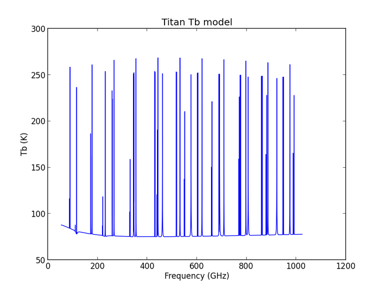
Titan
Model from Mark Gurwell, from 53.3-1024.1 GHz. Contains surface and atmospheric emission. The atmosphere includes N2-N2 and N2-CH4 Collision-Induced Absorption (CIA), and lines from minor species CO, 13CO, C18O, HCN, H13CN and HC15N. See, e.g., Gurwell & Muhleman (2000) [8]; Gurwell (2004) [9].
Asteroids
Some asteroids, namely Ceres, Pallas, Vesta, and Juno are included in the Butler-JPL-Horizons 2012. The models consists of the constant brightness temperature in frequency. For Ceres, Pallas, and Vesta, updated models based on thermophysical models (TPM) (T. Mueller, private communication) which are tabulated in time and frequency, are available for the observations taken after January 1st 2015, 0:00 UT. setjy task will automatically switch to the new models for the observations taken on and after that date. The TPM are also available for Lutetia but it is not advised to use for the absolute flux calibration for ALMA. Each of the tabulated models contains the flux density at 30, 80, 115, 150, 200, 230, 260, 300, 330, 360, 425, 650, 800, 950, and 1000 GHz. The time resolution is 1 hour for Ceres and 15 min for Lutetia, Pallas, and Vesta. The cubic interpolation is employed to obtain the flux densities at other frequencies. The models for Ceres, Pallas, and Vesta were recently updated to cover the period of January 1st 2026 to December 31, 2026. Extending these models beyond 2026 is in progress. The following is the detailed note on the recent update.
TPM prediction for ALMA observations of Ceres, Pallas, Vesta ------------------------------------------------------------ Thomas Mueller 23-Oct-2025 Model predictions for Ceres, Pallas, and Vesta are done for 2026, with either 1-hour (Ceres) or 15-min (Pallas, Vesta) time resolution: - Ceres_ALMA_TPMprediction_2026_1hour_v2.txt - Pallas_ALMA_TPMprediction_2026_15min.txt - Vesta_ALMA_TPMprediction_2026_15min.txt TPM solutions based on parameters & model concepts described in: Mueller, Balog, Nielbock et al.: "Herschel celestial calibration sources: Four large main-belt asteroids as prime flux calibrators for the far-IR/sub-mm range", Exp.Astr. 37, 253 (2014), DOI 10.1007/s10686-013-9357-y[ADS]. Recent updates of the models include the following aspects: 1) Ceres: - updated spin-shape solution by Vernazza et al. (2021) [ADS], based on high-resolution VLT-SPHERE measurements, and, as available from the DAMIT database (model 5915) - update on the global hemispherical spectral emissivity model, based on ALMA Band 7 measurements of Ceres (amplitude calibrator Uranus or Neptune) 2) Pallas: - updated H-G values from recent entries in the SSO Card, refering to Moskovitz et al., Ast. & Comp., 41, 100661 (2022) [ADS] - updated spin-shape solution by Marsset et al., Nature Astronomy 4, 569 (2020) [ADS], based on high-resolution VLT-SPHERE measurements, and, as available from the DAMIT database (model 4395) - update on the global hemispherical spectral emissivity model, based on ALMA Band 3,6,7,8 measurements of Pallas (amplitude calibrator Uranus or Neptune) 4) Vesta: - updated spin-shape solution by Vernazza et al. (2021) [ADS], based on high-resolution VLT-SPHERE measurements, and, as available from the DAMIT database (model 5920) - update on the global hemispherical spectral emissivity model, based on ALMA Band 3,6,7,8 measurements of Vesta (amplitude calibrator Uranus or Neptune) Monochromatic flux density predictions were made at the specified observation mid-times in the geocentric reference frame and for the reference frequencies of 29.9792, 91.501, 103.50, 232.99, 343.48, 999.31 GHz, corresponding to 10000.0, 3276.4, 2896.5, 1286.7, 872.8, and 300.0 um, respectively. For the final tables, the fluxes were interpolated (in log-log space) to obtain values at 30.0, 80.0, 115.0, 150.0, 200.0, 230.0, 260.0, 300.0, 330.0, 360.0, 425.0, 650.0, 800.0, 950.0, 1000.0 GHz. Note: a critical element for the submm/mm predictions is the description of the sub-surface emission. This is done via wavelength-dependent emissivity models which go back to the paper by Mueller & Lagerros, A&A 338, 340 (1998): "Asteroids as far-infrared photometric standards for ISOPHOT" [ADS], but have been updated after a careful investigation of available ALMA measurements with amplitude calibrator Uranus or Neptune (Ruediger Kneissel, Matias Radiszcz, 2025). The current model solutions are tested against the following ALMA measurements, taken between 2017 and 2025 (provided by Matias Radiszcz on 16-Oct-2025): Number of measurements: Band_3 Band_6 Band_7 Band_9 Ceres 0 0 134 0 Pallas 42 29 154 18 Vesta 134 26 184 18 Comparison between ALMA observations and model predictions (current version of the asteroid models): Obj Band f(ðœ¶)_corr AMPCAL_Ura AMCAL_Nep all_data Comment Ceres 7 No 1.04/1.05/0.026 1.01/1.02/0.049 1.02/1.03/0.046 v1 Ceres 7 Yes 1.00/1.00/0.019 1.00/0.99/0.031 1.00/1.00/0.027 v2 Pallas 9 No 0.99/0.98/0.043 1.03/1.03/0.049 1.00/1.00/0.047 -- Pallas 7 No 1.01/1.01/0.021 1.00/1.00/0.036 1.01/1.01/0.028 -- Pallas 6 No 0.98/0.98/0.024 1.00/0.99/0.049 0.99/0.98/0.042 -- Pallas 3 No 1.00/1.01/0.034 1.00/1.01/0.036 1.00/1.01/0.035 -- Vesta 9 No 0.98/0.99/0.055 1.01/0.99/0.069 1.00/0.99/0.066 -- Vesta 7 No 1.00/1.00/0.033 0.98/0.98/0.036 0.99/0.99/0.036 -- Vesta 6 No 0.98/0.99/0.038 0.98/0.99/0.031 0.98/0.99/0.033 -- Vesta 3 No 1.00/1.00/0.041 1.00/0.99/0.039 1.00/1.00/0.040 -- (see also ceres_all.tbl, pallas_all.tbl, vesta_all.tbl) Based on the above Observation-to-Model ratios and standard deviations, we assign an absolute model accuracy for all 3 objects, in the ALMA bands 3, 6, 7, 9 of better than 5%. There are plans to publish the available Ceres, Pallas, and Vesta measurements (in ALMA bands 3, 6, 7, and 9) together with the corresponding model predictions.
Ceres
Model with a constant \(T_b\) = 185K over frequencies (Moullet et al. 2010 [10], Muller & Lagerros 2002 [11], Redman et al. 1998 [12], Altenhoff et al. 1996 [13]) if time of the observations took place (\(t_{obs}\)) is before 2015.01.01, 0:00 UT, TPM if \(t_{obs}\) \(\ge\) 2015.01.01, 0:00 UT.
Pallas
Model with a constant \(T_b\) = 189K (Chamberlain et al. 2009 [14], Altenhoff et al. 1994 [15]) for \(t_{obs}\) \(\lt\) 2015.01.01, 0:00 UT, and TPM for \(t_{obs}\) \(\ge\) 2015.01.01, 0:00 UT
Vesta
Model with a constant \(T_b\) = 155K (Leyrat et al. 2012 [16], Chamberlain et al. 2009 [14], Redman et al. 1998 [12], Altenhoff et al. 1994 [15]) for \(t_{obs}\) \(\lt\) 2015.01.01, 0:00 UT, and TPM for \(t_{obs}\) \(\ge\) 2015.01.01, 0:00 UT
Juno
Model with a constant \(T_b\) = 153K (Chamberlain et al. 2009 [14], Altenhoff et al. 1994 [15])
Bibliography
Baars, J. W. M. et al. 1977, A&A, 61, 99 ADS
Kellermann, K. I. 2009, A&A 500, 143 ADS
Perley, R. A., & Butler, B. J. 2013, ApJS, 204, 19 ADS
Scaife, A. M., & Heald, G. H. 2012, MNRAS, 423, 30 ADS
Partridge et al. 2016, ApJ 821,1 ADS
Clancy, R.T. et al. 2012, Icarus, 217, 779 ADS
Perley, R. A. & Butler, B. J. 2017, ApJS, 230,7ADS
Rudy, D.J. et al. 1987, Icarus, 71, 159 ADS
Gurwell, M.A. & D.O. Muhleman 2000, Icarus, 145, 65w ADS
Gurwell, M.A. 2004, ApJ, 616, L7 ADS
Moullet, A. et al. 2010, A&A, 516, L10 ADS
Muller, T.G. & J.S.V. Lagerros 2002, A&A, 381, 324 ADS
Redman, R.O. et al. 1998, AJ, 116, 1478 ADS
Altenhoff, W.J. et al. 1996, A&A, 309, 953 ADS
Chamberlain, M.A. et al. 2009, Icarus, 202, 487 ADS
Altenhoff, W.J. et al. 1994, A&A, 287, 641 ADS
Leyrat, C. et al. 2012, A&A, 539, A154 ADS
Flux Calibrator Models - Data Formats
Conventions and Data Formats
This section describes the conventions, the formats as well as the locations of the data of the flux density calibrator models used in setjy. The detailed descriptions of specific flux standards and list of the calibrators are found in Flux Calibrator Models in the Reference Material section.
Extragalactic flux calibrator source models
The spectral flux density models are expressed in a polynomial in the form
where \(\nu\) is a frequency either in MHz or GHz depending on the standard. In setjy, the point source model is constructed as a componentlist scaled by the spectral flux density model. For the standards, Baars, Perley 90, Perley-Taylor 95, Perley-Taylor 99, Perley-Butler 2010, and Stevens-Reynolds 2016,the polynomial coefficients are hard-coded in the code.
For Perley-Butler 2013 and Scaife-Heald 2012, the coefficients are stored in CASA tables called PerleyButler2013Coeffs and ScaifeHeald2012Coeffs, respectively located in ~/nrao/VLA/standards/ in the CASA data directory(from CASA prompt, you can find the data root path by typing casa[‘dirs’][‘data’]). The separation of the data from the flux calibration code makes the maintenace easy and enable a user to acces the informaiton directly. Your can access these tables using the table tool (tb) and browsetable task. The list of the column header for PerleyButler2013Coeffs is shown below:
CASA <8>: tb.colnames
--------> tb.colnames()
Out[8]:
['Epoch',
'3C48_coeffs',
'3C48_coefferrs',
'3C138_coeffs',
'3C138_coefferrs',
'3C147_coeffs',
'3C147_coefferrs',
'3C286_coeffs',
'3C286_coefferrs',
'3C123_coeffs',
'3C123_coefferrs',
'3C295_coeffs',
'3C295_coefferrs',
'3C196_coeffs',
'3C196_coefferrs']
The coefficients of each source are stored in a column as a vector and the corresponding errors are stored in a seperate column. The different row represents the corresponding coefficinets at that epoch for the time variable sources while for the steady sources each row contains identical information. The frequency is assumed in GHz.
The list of the column header for ScaifeHeald2012Coeffs is shown below:
CASA <11>: tb.colnames
---------> tb.colnames()
Out[11]:
['Epoch',
'3C48_coeffs',
'3C48_coefferrs',
'3C147_coeffs',
'3C147_coefferrs',
'3C196_coeffs',
'3C196_coefferrs',
'3C286_coeffs',
'3C286_coefferrs',can b
'3C295_coeffs',
'3C295_coefferrs',
'3C380_coeffs',
'3C380_coefferrs']
The reference frequnecy for Scaife-Heald 2012 is 150MHz.
Solar System objects
For the solar system object used as a flux calibrator, setjy contstruct a model visibiity of the calibrator with the (averaged) brightness temperature model and ephemeris data of the sources as described in ALMA Memo #594. While the older Bulter-JPL-Horizons 2010 standard, hard-coded the brightness temperature models in the code, the models for Butler-JPL-Horizons 2012 are tabulated in ASCII files (SSobject_name_Tb.dat) located in the CASA data directory under ~/alma/SolarSystemModels. With an exception of Mars, the data for the brightness temparature models are stored in a simple format: 1st column - source frequency in GHz; 2nd column - the brightness temperature in Kelvin. The follow example script shows how it can be plotted for Titan.
import numpy as np

rootdatapath=casa['dirs']['data']
source='Titan'
datapath=rootdatapath+'/alma/SolarSystemModels/'+source+'_Tb.dat'
data=np.genfromtxt(datapath)
data=data.transpose()

freq=data[0]
temp=data[1]
pl.plot(freq,temp)
pl.title(source+' Tb model')
pl.xlabel('Frequency (GHz)')
pl.ylabel('Tb (K)')
And the following is the output plot by executing the script above.
The Tb model for Mars (Mars_Tb.dat) is calculated as a function of time and frequency, with tabulations every hour and at frequencies of: 30, 80, 115, 150, 200, 230, 260, 300, 330, 360, 425, 650, 800, 950, and 1000 GHz. The first line of the file contain frequencies in GHz. The data starts at the second line of the file with the format: YYYY MM DD HH MJD Tb for at each frequency sepearated by a space.
New Asteroid models
Ceres_fd_time.dat, Luthetia_fd_time.dat, Pallas_fd_time.dat, and Vesta_fd_time.dat contain thermophysical models by Th. Mueller (private communication). These time variable models are already converted to flux densities and are tabulated for 30, 80, 115, 150, 200, 230, 260, 300, 330, 360, 425, 650, 800, 950, and 1000 GHz. Time intevals are 1 hr. for Ceres and 15min. for Luthetia, Pallas, and Vesta with the data available from 2015 01 01 0UT to 2021 01 01 0 UT. In setjy task,these models are automatically selected for the data with the observation dates falls within this time range.
Spectral Frames
Spectral Frames supported in CASA
Spectral Frames
CASA supported spectral frames:
Frame |
Description |
Definition |
|---|---|---|
REST |
rest frequency |
Lab frame or source frame; cannot be converted to any other frame |
LSRK |
LSR as a kinematic (radio) definition (J2000) based on average velocity of stars in the Solar neighborhood |
20km/s in direction of RA, Dec - [270,+30] deg (B1900.0) (Gordon 1975 [1] ) |
LSRD |
Local Standard of Rest (J2000), dynamical, IAU definition. Solar peculiar velocity in the reference frame of a circular orbit about the Galactic Center, based on average velocity of stars in the Solar neighborhood and solar peculiar motion |
U\(\odot\)=9kms/s, V\(\odot\)=12km/s,W\(\odot\)=7km/s. Or 16.552945km/s towards l,b = 53.13, +25.02 deg (Delhaye 1965 [2]) |
BARY |
Solar System Baryceneter (J2000) |
|
GEO |
Geocentric, referenced to the Earth’s center |
|
TOPO |
Topocentric |
Local observatory frame, fixed in observing frequency, no doppler tracking |
GALACTO |
Galactocentric (J2000), referenced to dynamical center of the Galaxy |
220 km/s in the direction l,b = 270, +0 deg. (Kerr and Lynden-Bell 1986 [3]) |
LGROUP |
Mean motion of Local Group Galaxies with respect to its bary center |
308km/s towards l,b = 105,-7 |
CMB |
Cosmic Microwave Background, COBE measurements of dipole anisotropy |
369.5km/s towards l,b = 264.4,48.4. (Kogut et al. 1993 [4]) |
Undefined |
Doppler Types
CASA supported Doppler types (velocity conventions) where \(f_v\) is the observed frequency and \(f_0\) is the rest frame frequency of a given lineand positive velocity V is increasing away from the observer:
Name |
Description |
|---|---|
RADIO |
\(V = c \frac{(f_0 - f_v)}{f_0}\) |
Z |
\(V=cz\) \(z = \frac{(f_0 - f_v)}{f_v}\) |
RATIO |
\(V=c(\frac{f_v}{f_o})\) |
BETA |
\(V=c\frac{(1-(\frac{f_v}{f_0})^2)}{(1+(\frac{f_v}{f_0})^2)}\) |
GAMMA |
\(V=c\frac{(1 + (\frac{f_v}{f_0})^2)}{2\frac{f_v}{f_0}}\) |
OPTICAL |
\(V= c\frac{(f_0 - f_v)}{f_v}\) |
TRUE |
\(V=c\frac{(1-(\frac{f_v}{f_0})^2)}{(1+(\frac{f_v}{f_0})^2)}\) |
RELATIVISTIC |
\(V=c\frac{(1-(\frac{f_v}{f_0})^2)}{(1+(\frac{f_v}{f_0})^2)}\) |
Bibliography
Gordon 1975: “Methods of Experimental Physics: Volume 12: Astrophysics, Part C: Radio Observations”, ed. M.L.Meeks, Academic Press 1976
Delhaye 1965 (
Kerr F. J. & Lynden-Bell D. 1986 MNRAS, 221, 1023 (
Kogut A. et al. 1993 ( ^
Time Reference Frames
CASA supported time reference frames:
Acronym |
Name |
Description |
|---|---|---|
ET |
Ephemeris Time |
The time scale used prior to 1984 as the independent variable in gravitational theories of the solar system. In 1984, ET was replaced by dynamical time (see TDB, TT). |
GAST |
Greenwich Apparent Sidereal Time |
The Greenwich hour angle of the true equinox [1] of date. |
GMST |
Greenwich Mean Sidereal Time |
The Greenwich hour angle of the mean equinox [1] of date, defined as the angular distance on the celestial sphere measured westward along the celestial equator from the Greenwich meridian to the hour circle that passes through a celestial object or point. GMST (in seconds at UT1=0) = 24110.54841 + 8640184.812866 * T + 0.093104 * \(T^2\) - 0.0000062 * \(T^3\) where T is in Julian centuries from 2000 Jan. 1 12h UT1: T = d / 36525 d = JD - 2451545.0 |
GMST1 |
GMST calculated specifically with reference to UT1 |
|
IAT |
International Atomic Time (a.k.a. TAI en Francais): |
The continuous time scale resulting from analysis by the Bureau International des Poids et Mesures of atomic time standards in many countries. The fundamental unit of TAI is the SI second [2] on the geoid [3] , and the epoch is 1958 January 1. |
LAST |
Local Apparent Sidereal Time |
LAST is derived from LMST by applying the equation of equinoxes [1] or nutation of the mean pole of the Earth from mean to true position yields LAST. |
LMST |
Local Mean Sidereal Time |
Sidereal time is the hour angle of the vernal equinox, the ascending node of the ecliptic on the celestial equator. The daily motion of this point provides a measure of the rotation of the Earth with respect to the stars, rather than the Sun. It corresponds to the coordinate right ascension of a celestial body that is presently on the local meridian. LMST is computed from the current GMST plus the local offset in longitude measured positive to the east of Greenwich, (converted to a sidereal offset by the ratio 1.00273790935 of the mean solar day to the mean sidereal day.) LMST = GMST + (observer’s east longitude) |
TAI |
International Atomic Time (a.k.a. TAI en Francais) |
see IAT |
TCB |
Barycentric Coordinate Time |
The coordinate time of the Barycentric Celestial Reference System (BCRS), which advances by SI seconds [2] within that system. TCB is related to TCG and TT by relativistic transformations that include a secular term. |
TCG |
||
TDB |
Barycentric Dynamical Time |
A time scale defined by the IAU (originally in 1976; named in 1979; revised in 2006) used in barycentric ephemerides and equations of motion. TDB is a linear function of TCB that on average tracks TT over long periods of time; differences between TDB and TT evaluated at the Earth’s surface remain under 2 ms for several thousand years around the current epoch. TDB is functionally equivalent to Teph, the independent argument of the JPL planetary and lunar ephemerides DE405/LE405. |
TDT |
Terrestrial Dynamical Time |
The time scale for apparent geocentric ephemerides defined by a 1979 IAU resolution. In 1991 it was replaced by TT. |
TT |
Terrestrial Time |
An idealized form of International Atomic Time (TAI) with an epoch offset; in practice TT = TAI + 32s.184. TT thus advances by SI seconds on the geoid [3] |
UT |
Universal Time |
Loosely, mean solar time on the Greenwich meridian (previously referred to as Greenwich Mean Time). In current usage, UT refers either to UT1 or to UTC. |
UT1 |
UT1 is formally defined by a mathematical expression that relates it to sidereal time. Thus, UT1 is observationally determined by the apparent diurnal motions of celestial bodies, and is affected by irregularities in the Earth’s rate of rotation. |
|
UT2 |
Before 1972 the time broadcast services kept their time signals within 0.1 seconds [2] of UT2, which is UT1 with annual and semiannual variations in the earth’s rotation removed. The formal relation between UT1 and UT2 is UT2 = UT1 + 0.022 * sin(2 * Pi * t) - 0.012 * cos(2 * Pi * t) 0.006 * sin(4 * Pi * t) + 0.007 * cos(4 * Pi * t) where t = 2000.0 + (MJD - 51544.03) / 365.2422 is the Besselian day fraction, and MJD is the Modified Julian Date (Julian Date - 2400000.5) |
|
UTC |
Coordinated Universal Time |
UTC is based on IAT but is maintained within 0s.9 of UT1 by the introduction of leap seconds when necessary. |
Footnote(s)
mean equator and equinox v. true equator and equinox: The mean equator and equinox are used for the celestial coordinate system defined by the orientation of the Earth’s equatorial plane on some specified date together with the direction of the dynamical equinox on that date, neglecting nutation. Thus, the mean equator and equinox moves in response only to precession. Positions in a star catalog have traditionally been referred to a catalog equator and equinox that approximate the mean equator and equinox of a standard epoch. The true equator and equinox are affected by both precession and nutation. The Equation of the Equinoxes is the difference (apparent sidereal time minus mean sidereal time). Equivalently, the difference between the right ascensions of the true and mean equinoxes, expressed in time units.
The Systeme International (SI) second is defined as the duration of 9,192,631,770 cycles of radiation corresponding to the transition between two hyperfine levels of the ground state of caesium 133.
The geoid is an equipotential surface that coincides with mean sea level in the open ocean. On land it is the level surface that would be assumed by water in an imaginary network of frictionless channels connected to the ocean.
Coordinate Frames
CASA supported spatial coordinate frames:
Name |
Description |
|---|---|
J2000 |
mean equator and equinox at J2000.0 (FK5) |
JNAT |
geocentric natural frame |
JMEAN |
mean equator and equinox at frame epoch |
JTRUE |
true equator and equinox at frame epoch |
APP |
apparent geocentric position |
B1950 |
mean epoch and ecliptic at B1950.0. |
B1950_VLA |
mean epoch (1979.9) and ecliptic at B1950.0 |
BMEAN |
mean equator and equinox at frame epoch |
BTRUE |
true equator and equinox at frame epoch |
GALACTIC |
Galactic coordinates |
HADEC |
topocentric HA and declination |
AZEL |
topocentric Azimuth and Elevation (N through E) |
AZELSW |
topocentric Azimuth and Elevation (S through W) |
AZELNE |
topocentric Azimuth and Elevation (N through E) |
AZELGEO |
geodetic Azimuth and Elevation (N through E) |
AZELSWGEO |
geodetic Azimuth and Elevation (S through W) |
AZELNEGEO |
geodetic Azimuth and Elevation (N through E) |
ECLIPTC |
ecliptic for J2000 equator and equinox |
MECLIPTIC |
ecliptic for mean equator of date |
TECLIPTIC |
ecliptic for true equator of date |
SUPERGAL |
supergalactic coordinates |
ITRF |
coordinates wrt ITRF Earth frame |
TOPO |
apparent topocentric position |
ICRS |
International Celestial reference system |
Physical Units
CASA regonizes physical units as listed in the following Tables.
Prefix Name Value ——–>Physical units: Prefixes
Unit |
Name |
Value |
|---|---|---|
$ |
(currency) |
1 _ |
% |
(percent) |
0.01 |
%% |
(permille) |
0.001 |
A |
(ampere) |
1 A |
AE |
(astronomical unit) |
149597870659 m |
AU |
(astronomical unit) |
149597870659 m |
Bq |
(becquerel) |
1 s−1 |
C |
(coulomb) |
1 s A |
F |
(farad) |
1 m−2 kg−1 s4 A2 |
Gy |
(gray) |
1 m2 s−2 |
H |
(henry) |
1 m2 kg s−2 A−2 |
Hz |
(hertz) |
1 s−1 |
J |
(joule) |
1 m2 kg s−2 |
Jy |
(jansky) |
10−26 kg s−2 |
K |
(kelvin) |
1 K |
L |
(litre) |
0.001 m3 |
M0 |
(solar mass) |
1.98891944407× 1030 kg |
N |
(newton) |
1 m kg s−2 |
Ohm |
(ohm) |
1 m2 kg s−3 A−2 |
Pa |
(pascal) |
1 m−1 kg s−2 |
S |
(siemens) |
1 m−2 kg−1 s3 A2 |
S0 |
(solar mass) |
1.98891944407× 1030 kg |
Sv |
(sievert) |
1 m2 s−2 |
T |
(tesla) |
1 kg s−2 A−1 |
UA |
(astronomical unit) |
149597870659 m |
V |
(volt) |
1 m2 kg s−3 A−1 |
W |
(watt) |
1 m2 kg s−3 |
Wb |
(weber) |
1 m2 kg s−2 A−1 |
_ |
(undimensioned) |
1 _ |
a |
(year) |
31557600 s |
arcmin |
(arcmin) |
0.000290888208666 rad |
arcsec |
(arcsec) |
4.8481368111×10⁻⁶ rad |
as |
(arcsec) |
4.8481368111e×10−6 rad |
cd |
(candela) |
1 cd |
cy |
(century) |
3155760000 s |
d |
(day) |
86400 s |
deg |
(degree) |
0.0174532925199 rad |
g |
(gram) |
0.001 kg |
h |
(hour) |
3600 s |
l |
(litre) |
0.001 m3 |
lm |
(lumen) |
1 cd sr |
lx |
(lux) |
1 m−2 cd sr |
m |
(metre) |
1 m |
min |
(minute) |
60 s |
mol |
(mole) |
1 mol |
pc |
(parsec) |
3.08567758065×10¹⁶ m |
rad |
(radian) |
1 rad |
s |
(second) |
1 s |
sr |
(steradian) |
1 sr |
t |
(tonne) |
1000 kg |
Physical SI Units
Unit |
Name |
Value |
|---|---|---|
“ |
(arcsec) |
4.8481368111×10⁻⁶ rad |
“_2 |
(square arcsec) |
2.35044305391× 10⁻¹¹ sr |
‘ |
(arcmin) |
0.000290888208666 rad |
‘_2 |
(square arcmin) |
8.46159499408×10⁻⁸ sr |
: |
(hour) |
3600 s |
:: |
(minute) |
60 s |
Ah |
(ampere hour) |
3600 s A |
Angstrom |
(angstrom) |
1e-10 m |
Btu |
(British thermal unit (Int)) |
1055.056 m2 kg s−2 |
CM |
(metric carat) |
0.0002 kg |
Cal |
(large calorie (Int)) |
4186.8 m2 kg s−2 |
FU |
(flux unit) |
10−26 kg s−2 |
G |
(gauss) |
0.0001 kg s−2 A−1 |
Gal |
(gal) |
0.01 m s−2 |
Gb |
(gilbert) |
0.795774715459 A |
Mx |
(maxwell) |
10−8 m2 kg s−2 A−1 |
Oe |
(oersted) |
79.5774715459 m−1 A |
R |
(mile) |
0.000258 kg−1 s A |
St |
(stokes) |
0.0001 m2 s−1 |
Torr |
(torr) |
133.322368421 m−1 kg s−2 |
USfl_oz |
(fluid ounce (US)) |
2.95735295625×10⁻⁵ m3 |
USgal |
(gallon (US)) |
0.003785411784 m3 |
WU |
(WSRT flux unit) |
5× 10⁻²⁹ kg s−2 |
abA |
(abampere) |
10 A |
abC |
(abcoulomb) |
10 s A |
abF |
(abfarad) |
109 m−2 kg−1 s4 A2 |
abH |
(abhenry) |
10−9 m2 kg s−2 A−2 |
abOhm |
(abohm) |
10−9 m2 kg s−3 A−2 |
abV |
(abvolt) |
10−8 m2 kg s−3 A−1 |
ac |
(acre) |
4046.8564224 m2 |
arcmin_2 |
(square arcmin) |
8.46-2159499408×10−8 sr |
arcsec_2 |
(square arcsec) |
2.35044305391×10⁻¹¹ sr |
ata |
(technical atmosphere) |
98066.5 m−1.kg.s−2 |
atm |
(standard atmosphere) |
101325 m−1.kg.s−2 |
bar |
(bar) |
100000 m−1.kg.s−2 |
beam |
(undefined beam area) |
1 _ |
cal |
(calorie (Int)) |
4.1868 m2 kg s−2 |
count |
(count) |
1 _ |
cwt |
(hundredweight) |
50.80234544 kg |
deg_2 |
(square degree) |
0.000304617419787 sr |
dyn |
(dyne) |
10−5 m kg s−2 |
eV |
(electron volt) |
1.60217733×10⁻¹⁹ m2 kg s−2 |
erg |
(erg) |
10−7 m2 kg s−2 |
fl_oz |
(fluid ounce (Imp)) |
2.84130488996×10⁻⁵ m3 |
ft |
(foot) |
0.3048 m |
fu |
(flux unit) |
10−26 kg s−2 |
fur |
(furlong) |
201.168 m |
gal |
(gallon (Imp)) |
0.00454608782394 m3 |
ha |
(hectare) |
10000 m2 |
hp |
(horsepower) |
745.7 m2 kg s−3 |
in |
(inch) |
0.0254 m |
kn |
(knot (Imp)) |
0.514773333333 m s−1 |
lambda |
(lambda) |
1 _ |
lb |
(pound (avoirdupois)) |
0.45359237 kg |
ly |
(light year) |
9.46073047×10¹⁵ m |
mHg |
(metre of mercury) |
133322.387415 m−1 kg s−2 |
mile |
(mile) |
1609.344 m |
n_mile |
(nautical mile (Imp)) |
1853.184 m |
oz |
(ounce (avoirdupois)) |
0.028349523125 kg |
pixel |
(pixel) |
1 _ |
sb |
(stilb) |
10000 m−2 cd |
sq_arcmin |
(square arcmin) |
8.46159499408×10⁻⁸ sr |
sq_arcsec |
(square arcsec) |
2.35044305391×10⁻¹¹ sr |
sq_deg |
(square degree) |
0.000304617419787 sr |
statA |
(statampere) |
3.33564095198×10⁻¹⁰ A |
statC |
(statcoulomb) |
3.33564095198×10⁻¹⁰ s A |
statF |
(statfarad) |
1.11188031733×10⁻¹² m−2 kg−1 s4 A2 |
statH |
(stathenry) |
899377374000 m2 kg s−2 A−2 |
statOhm |
(statohm) |
899377374000 m2 kg s−3 A−2 |
statV |
(statvolt) |
299.792458 m2 kg s−3 A−1 |
u |
(atomic mass unit) |
1.661×10⁻²⁷ kg |
yd |
(yard) |
0.9144 m |
yr |
(year) |
31557600 s |
Custom units available in CASA
Physical Constants
Physical constants recognized by CASA
The physical constants listed below are defined in CASA. They can be listed with the command
import casatools.constants
print qa.map('Constants')
For information about the constants as stored in the code, please see this Casacore document
Constant |
Name |
Value |
|---|---|---|
pi |
3.14.. |
3.14159 |
ee |
2.71.. |
2.71828 |
c |
speed of light |
2.99792×10⁸ m s−1 |
G |
grav. constant |
6.67259×10¹¹ N m2 kg−2 |
h |
Planck constant |
6.62608×10⁻³⁴ J s |
HI |
HI line frequency |
1420.41 MHz |
R |
gas constant |
8.31451 J K−1 mol−1 |
NA |
Avogadro # |
6.02214×10²³ mol−1 |
e |
electron charge |
1.60218×10⁻¹⁹ C |
mp |
proton mass |
1.67262×10⁻²⁷ kg |
mp_me |
mp/me |
1836.15 |
mu0 |
permeability vac. |
1.25664×10⁻⁶ H m−1 |
eps0 |
permittivity vac. |
8.85418782×10⁻¹² F m-1 |
k |
Boltzmann constant |
1.38066×10⁻²³ J K−1 |
F |
Faraday constant |
96485.3 C mol−1 |
me |
electron mass |
9.10939×10⁻³¹ kg |
re |
electron radius |
2.8179e×10−15 m |
a0 |
Bohrs radius |
5.2918×10⁻¹¹ m |
R0 |
solar radius |
6.9599×10⁸ m |
k2 |
IAU grav. const2 |
0.000295912 AU3 d−2 S0−1 |
Resources and Links
Useful supplementary information relevant to CASA
Tutorials
CASAguides contains the most comprehensive data reduction tutorials for ALMA (including simulations) and the VLA. Tutorials also exist for other telescopes, such as ATCA, SMA, and CARMA. The CASAguides wiki is also a great resource for tips and tricks in using CASA and contains user contributed scripts.
Workshops
ALMA community days webpages provide material that was used during workshops
The 2018 VLA data reduction workshop contains course material
Synthesis Imaging in Radio Astronomy II (pdf book (chapters)
Python
Science Data Model
The SDM description and SDM definition document can be found on this page