plotcal

plotcal(caltable, xaxis='', yaxis='', poln='', field='', antenna='', spw='', timerange='', subplot=111, overplot=False, clearpanel='Auto', iteration='', plotrange=[], showflags=False, plotsymbol='o', plotcolor='blue', markersize=5.0, fontsize=10.0, showgui=True, figfile='')

An all-purpose plotter for calibration results (Deprecated in CASA 5.8. Not present in CASA 6.2. Use plotms instead.)

[Description] [Examples] [Development] [Details]

Parameters

• caltable (string)

• xaxis (string=’’)

• yaxis (string=’’)

• poln (string=’’)

• field (string=’’)

• antenna (string=’’)

• spw (string=’’)

• timerange (string=’’)

• subplot (int=111)

• overplot (bool=False)

• clearpanel (string=’Auto’)

• iteration (string=’’)

• plotrange (doubleArray=[

  ])

• showflags (bool=False)

• plotsymbol (string=’o’)

• plotcolor (string=’blue’)

• markersize (double=5.0)

• fontsize (double=10.0)

• showgui (bool=True)

• figfile (string=’’)

Description

Most of the functionality of plotcal is now implemented in plotms.

We recommend the use of plotms for plotting calibration tables, except for certain VLBI cases that still need plotcal. Plotcal will be deprecated in the near future.

The plotcal task is available for examining solutions of all of the basic solvable types.

Warning

Alert: Currently, plotcal needs to know the MS from which caltable was derived to get indexing information. It does this using the name stored inside the table, which does not include the full path, but assumes the MS is in the current working directory. Thus if you are using a MS in a directory other than the current one, it will not find it. You need to change directories using cd in IPython (or os.chdir() inside a script) to the MS location. If the MS is not found, plotcal wil plot solutions, but ignore any specified selection.

Parameter descriptions

caltable

Specify the name of the calibration table to be plotted as a string in caltable.

Axis choices: xaxis, yaxis

Specify the axes to be plotted in xaxis and yaxis. The possible choices are listed in the Parameters section.

General selection: field, spw, antenna, timerange

The plotcal task uses the same selection syntax as the solving tasks for these parameters. See here for more information.

Polarization selection: poln

The poln parameter determines what polarization or combination of polarizations is being plotted. Choosing poln=’RL’ plots both R and L polarizations on the same plot. The respective XY options do equivalent things. The poln=’/’ option plots amplitude ratios or phase differences between whatever polarizations are in the MS (R and L or X and Y).

Plot control: subplot, iteration, overplot, plotrange

The subplot parameter is particularly helpful in making multi-panel plots. The format is subplot=yxn where yxn is an integer with digit y representing the number of plots in the y-axis, digit x the number of panels along the x-axis, and digit n giving the location of the plot in the panel array (where n = 1, …, xy, in order upper left to right, then down).

The iteration parameter allows you to select an identifier to iterate over when producing multi-page or multi-panel plots. The choices for iteration are: ‘antenna’, ‘time’, ‘spw’, ‘field’. For example, if per-antenna solution plots are desired, use iteration=’antenna’. You can then use subplot to specify the number of plots to appear on each page. In this case, set the n to 1 in subplot=yxn. Use the Next button on the plotcal window to advance to the next set of plots. Note that iteration can take more than one choice (as a single string containing a comma-separated list of the options). When specifying multiple iteration axes, the iteration order will be fixed (independent of the order specified in the iteration string). The iteration order (slowest to fastest) is iteration=’antenna,time,field,spw’.

The overplot parameter may be used to plot more than one execution of plotcal on the same plot surface. If overplot=T, and the specified plot axes are consistent, any existing plot will not be cleared before plotting. It can useful to use the plotsymbol parameter to change the plot symbols for different plotcal runs using overplot, so that the different solutions are distinguishable.

The range of the two axes can be specified in the plotrange parameter, as a list of real numbers in the following order:

plotrange=[xmin,xmax,ymin,ymax]

If the both values for either axis are zeros, the plot range on that axis will be set automatically.

Symbol control: plotsymbol, plotcolor, markersize, fontsize

Symbol type, color, and size, as well as fontsize for labels can be set with these parameters, which are adopted from the general matplotlib interface.

Plot files: showgui, figfile

If showgui=True, an interactive plot window will be generated to show the plot. If a filename is specified in figfile, a plot file will be generated. The format of the plotfile is indicated by a specified suffix on the filename; supported formats include emf, eps, pdf, png, ps, raw, rgba, svg, svgz.

Examples

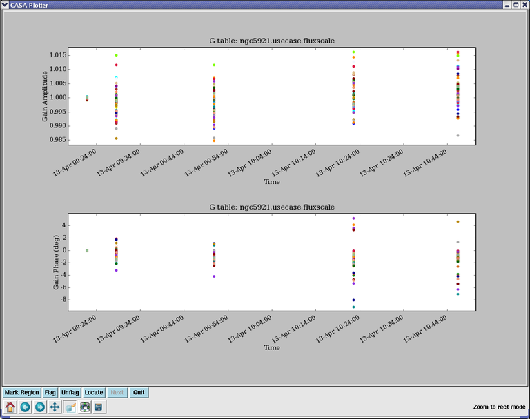
To plot amplitude and phase as a fuction of time on two panels of a single page, for ‘G’ solutions in a caltable called ‘ngc5121.usecase.fluxscale’:

plotcal(caltable='ngc5921.usecase.fluxscale',
        xaxis='time',yaxis = 'amp', subplot = 211)

plotcal(caltable='ngc5921.usecase.fluxscale',
        xaxis='time',yaxis = 'phase', subplot = 212)

The result is shown in the following figure:

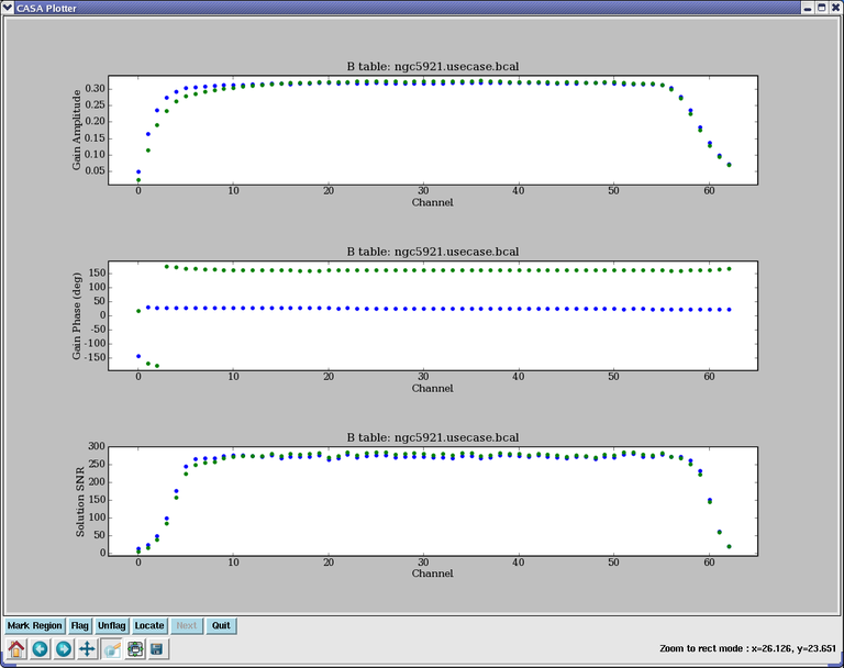
Similarly, to plot amplitude, phase and SNR as a function of frequency on a three-panel plot, for a ‘B’ solution for a single antenna stored in ‘ngc5921.usecase.bcal’:

plotcal(caltable='ngc5921.usecase.bcal',antenna='0', xaxis='freq',yaxis='amp', subplot=311)

plotcal(caltable='ngc5921.usecase.bcal',antenna='0', xaxis='freq',yaxis='phase', subplot=312)

plotcal(caltable='ngc5921.usecase.bcal',antenna='0', xaxis='freq',yaxis='snr', subplot=313)

This will generate the following figure:

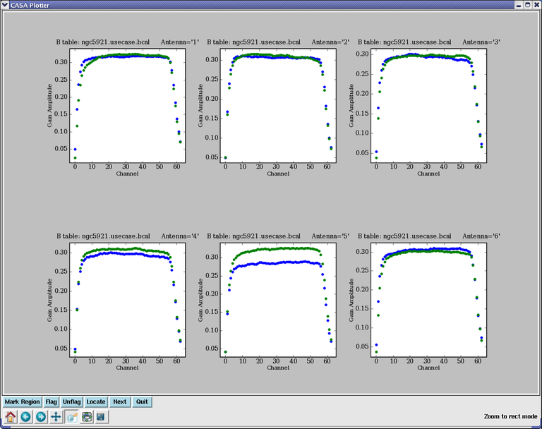
To show one amplitude vs. freq bandpass per plot, with 6 plots per page, iterating over antennas:

plotcal(caltable='ngc5921.usecase.bcal',antenna='0', xaxis='freq',yaxis='amp',
        iteration='antenna',subplot=231)

This will generate the following figure:

Development

No additional development details

Parameter Details

Detailed descriptions of each function parameter

caltable (string) - Name of input calibration table

xaxis (string='') - Value to plot along x axis (time,chan,freq, antenna,antenna1,antenna2,scan, amp,phase,real,imag,snr, tsys,delay,rate,disp,spgain)

yaxis (string='') - Value to plot along y axis (amp,phase,real,imag,snr, antenna,antenna1,antenna2,scan, tsys,delay,rate,disp,spgain,tec)

poln (string='') - Antenna polarization to plot (RL,R,L,XY,X,Y,/)

field (string='') - field names or index of calibrators: ''==>all

antenna (string='') - antenna/baselines: ''==>all, antenna = '3,VA04'

spw (string='') - spectral window:channels: ''==>all, spw='1:5~57'

timerange (string='') - time range: ''==>all

subplot (int=111) - Panel number on display screen (yxn)

overplot (bool=False) - Overplot solutions on existing display

clearpanel (string='Auto') - Specify if old plots are cleared or not (ignore)

iteration (string='') - Iterate plots on antenna,time,spw,field

plotrange (doubleArray=[ ]) - plot axes ranges: [xmin,xmax,ymin,ymax]

showflags (bool=False) - If true, show flagged solutions

plotsymbol (string='o') - pylab plot symbol

plotcolor (string='blue') - initial plotting color

markersize (double=5.0) - Size of plotted marks

fontsize (double=10.0) - Font size for labels

showgui (bool=True) - Show plot on gui

figfile (string='') - ''= no plot hardcopy, otherwise supply name