Open in Colab: https://colab.research.google.com/github/casangi/casadocs/blob/master/docs/notebooks/synthesis_calibration.ipynb
Synthesis Calibration
This chapter explains how to calibrate interferometer data within the CASA task system. Calibration is the process of determining the net complex correction factors that must be applied to each visibility in order to make them as close as possible to what an idealized interferometer would measure, such that when the data is imaged an accurate picture of the sky is obtained. This is not an arbitrary process, and there is a philosophy behind the CASA calibration methodology. For the most part, calibration in CASA using the tasks is not too different than calibration in other packages such as AIPS or Miriad.
Calibration tasks
Alert: As part of continuing development of a more flexible and improved interface for specifying calibration for apply, a new parameter has been introduced in applycal and the solving tasks: docallib. This parameter toggles between use of the traditional calibration apply parameters ( gaintable, gainfield, interp, spwmap, and calwt), and a new callib parameter which currently provides access to the experimental Cal Library mechanism, wherein calibration instructions are stored in a file. The default remains docallib=False in CASA 4.5, and this reveals the traditional apply parameters which continue to work as always, and the remainder of this chapter is still written using docallib=False. Users interested in the Cal Library mechanism’s flexibility are encouraged to try it and report any problems; see here for information on how to use it, including how to convert traditional applycal to Cal Library format. Note also that plotms and mstransform now support use of the Cal Library to enable on-the-fly calibration when plotting and generating new MSs.
The standard set of calibration solving tasks (to produce calibration tables) are:
bandpass — complex bandpass (B) calibration solving, including options for channel-binned or polynomial solutions
gaincal — complex gain (G,T) and delay (K) calibration solving, including options for time-binned or spline solutions
fringefit — fringe-fitting solutions (usually for VLBI) that parameterize phase calibration with phase, delay, rate, and a dispersive term
polcal — polarization calibration including leakage, cross-hand phase, and position angle
blcal — baseline-based complex gain or bandpass calibration
There are helper tasks to create, manipulate, and explore calibration tables:
applycal — Apply calculated calibration solutions
clearcal — Re-initialize the calibration for a visibility dataset
fluxscale — Bootstrap the flux density scale from standard calibration sources
listcal — List calibration solutions
plotms — Plot calibration solutions
plotbandpass — Plot bandpass solutions
setjy — Compute model visibilities with the correct flux density for a specified source
smoothcal — Smooth calibration solutions derived from one or more sources
calstat — Statistics of calibration solutions
gencal — Create a calibration tables from metadata such as antenna position offsets, gaincurves and opacities
wvrgcal — Generate a gain table based on Water Vapor Radiometer data (for ALMA)
uvcontsub — Carry out uv-plane continuum fitting and subtraction
The Calibration Process
A work-flow diagram for CASA calibration of interferometry data is shown in the following figure. This should help you chart your course through the complex set of calibration steps. In the following sections, we will detail the steps themselves and explain how to run the necessary tasks and tools.
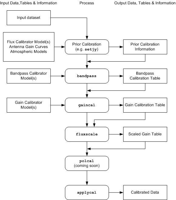
Flow chart of synthesis calibration operations. Not shown are use of table manipulation and plotting tasks: plotms and smoothcal
The process can be broken down into a number of discrete phases:
Calibrator Model Visibility Specification — set model visibilities for calibrators, either unit point source visibilities for calibrators with unknown flux density or structure (generally, sources used for calibrators are approximately point-like), or visibilities derived from a priori images and/or known or standard flux density values. Use the setjy task for calibrator flux densities and models.
Prior Calibration — set up previously known calibration quantities that need to be pre-applied, such antenna gain-elevation curves, atmospheric models, delays, and antenna position offsets. Use the gencal task for antenna position offsets, gaincurves, antenna efficiencies, opacity, and other prior calibrations
Bandpass Calibration — solve for the relative gain of the system over the frequency channels in the dataset (if needed), having pre-applied the prior calibration. Use the bandpass task
Gain Calibration — solve for the gain variations of the system as a function of time, having pre-applied the bandpass (if needed) and prior calibration. Use the gaincal task
Polarization Calibration — solve for polarization leakage terms and linear polarization position angle. Use the polcal task.
Establish Flux Density Scale — if only some of the calibrators have known flux densities, then rescale gain solutions and derive flux densities of secondary calibrators. Use the fluxscale task
Smooth — if necessary smooth calibration using the smoothcal task.
Examine Calibration — at any point, you can (and should) use plotms and/or listcal to look at the calibration tables that you have created
Apply Calibration to the Data — Corrected data is formed using the applycal task, and can be undone using clearcal
Post-Calibration Activities — this includes the determination and subtraction of continuum signal from line data (uvcontsub), the splitting of data-sets into subsets (split, mstransform), and other operations (such as simple model-fitting: uvmodelfit).
The flow chart and the above list are in a suggested order. However, the actual order in which you will carry out these operations is somewhat fluid, and will be determined by the specific data-reduction use cases you are following. For example, you may need to obtain an initial gain calibration on your bandpass calibrator before moving to the bandpass calibration stage. Or perhaps the polarization leakage calibration will be known from prior service observations, and can be applied as a constituent of prior calibration.
Calibration Philosophy
Calibration is not an arbitrary process, and there is a methodology that has been developed to carry out synthesis calibration and an algebra to describe the various corruptions that data might be subject to: the Hamaker-Bregman-Sault Measurement Equation (ME), described here. The user need not worry about the details of this mathematics as the CASA software does that for you. Anyway, it’s just matrix algebra, and your familiar scalar methods of calibration (such as in AIPS) are encompassed in this more general approach.
There are a number of ``physical’’ components to calibration in CASA:
data — in the form of the MeasurementSet (MS). The MS includes a number of columns that can hold calibrated data, model information, and weights
calibration tables — these are in the form of standard CASA tables, and hold the calibration solutions (or parameterizations thereof)
task parameters — sometimes the calibration information is in the form of CASA task parameters that tell the calibration tasks to turn on or off various features, contain important values (such as flux densities), or list what should be done to the data.
At its most basic level, Calibration in CASA is the process of taking “uncalibrated” data, setting up the operation of calibration tasks using task parameters, solving for new calibration tables, and then applying the calibration tables to form “calibrated” data. Iteration can occur as necessary, e.g., to re-solve for an eariler calibration table using a better set of prior calibration, often with the aid of other non-calibration steps (e.g. imaging to generate improved source models for “self-calibration”).
The calibration tables are the currency that is exchanged between the calibration tasks. The “solver” tasks (gaincal, bandpass, blcal, polcal) take in the MS (which may have a calibration model attached) and previous calibration tables, and will output an “incremental” calibration table (it is incremental to the previous calibration, if any). This table can then be smoothed using smoothcal if desired.
The final set of calibration tables represents the cumulative calibration and is what is applied to correct the data using applycal. It is important to keep track of each calibration table and its role relative to others. E.g., a provisional gain calibration solution will usually be obtained to optimize a bandpass calibration solve, but then be discarded in favor of a new gain calibration solution that will itself be optimized by use of the bandpass solution as a prior; the original gain calibration table should be discarded in this case. On the other hand, it is also permitted to generate a sequence of gain calibration tables, each relative to the last (and any other prior calibration used); in this case all relative tables should be carried forward through the process and included in the final applycal. It is the user’s responsibility to keep track of the role of and relationships between all calibration tables. Depending on the complexity of the observation, this can be a confusing business, and it will help if you adopt a consistent table naming scheme. In general, it is desirable to minimize the number of different calibration tables of a specific type, to keep the overall process as simple as possible and minimize the computational cost of applying them, but relative calibraition tables may sometimes be useful as an aid to understanding the origin and properties of the calibration effects. For example, it may be instructive to obtain a short time-scale gain calibraiton relative to a long time-scale one (e.g., obtained from a single scan) to approximatly separate electronic and atmospheric effects. Of course, calibration tables of different types are necessarily relative to each other (in the order in which they are solved).
Preparing for Calibration
A description of the range of prior information necessary to solve for calibration
There is a range of a priori information that may need to be initialized or estimated before calibration solving is carried out. This includes establishing prior information about the data within the MS:
weight initialization — if desired, initialization of spectral weights, using initweight (by default, unchannelized weight accounting is used, and no special action is required)
flux density models — establish the flux density scale using “standard” calibrator sources, with models for resolved calibrators, using setjy as well as deriving various prior calibration quanitities using various modes of gencal
gain curves — the antenna gain-elevation dependence
atmospheric optical depth — attenuation of the signal by the atmosphere, including correcting for its elevation dependence
antenna position errors — offsets in the positions of antennas assumed during correlation
ionosphere — dispersive delay and Faraday effects arising from signal transmission through the magnetized plasma of the ionosphere
switched power (EVLA) — electronic gains monitored by the EVLA online system
system temperature (ALMA) — turn correlation coefficient into correlated flux density (necessary for some telescopes)
generic cal factors — antenna-based amp, phase, delay
These are all pre-determined effects and should be applied (if known) as priors when solving for other calibration terms, and included in the final application of all calibration. If unknown, then they will be solved for or subsumed in other calibration such as bandpass or gains.
Each of these will now be described in turn.
Weight Initialization
See the section on data weights for a more complete description of weight accounting in CASA.
CASA 4.3 introduced initial experimental support for spectral weights. At this time, this is mainly relevant to ALMA processing for which spectral \(T_{sys}\) corrections, which faithfully reflect spectral sensitivity, are available. In most other cases, sensitivity is, to a very good approximation, channel-independent after bandpass calibration (and often also before), except perhaps at the very edges of spectral windows (and for which analytic expressions of the sensitivity loss are generally unavailable). Averaging of data with channel-dependent flagging which varies on sufficiently short timescales will also generate channel-dependent net weights (see split or mstransform for more details).
By default, CASA’s weight accounting scheme maintains unchannelized weight information that is appropriately updated when calibration is applied. In the case of spectral calibrations (\(T_{sys}\) and bandpass), an appropriate spectral average is used for the weight update. This spectral average is formally correct for weight update by bandpass. For \(T_{sys}\), traditional treatments used a single measurement per spectral window; ALMA has implemented spectral \(T_{sys}\) to better track sensitivity as a function of channel, and so should benefit from spectral weight accounting as described here, especially where atmospheric emmission lines occur. If spectral weight accounting is desired, users must re-initialize the spectral weights using the initweights task:
initweights(vis='mydata.ms', wtmode='nyq', dowtsp=True)
In this task, the wtmode parameter controls the weight initialization convention. Usually, when initializing the weight information for a raw dataset, one should choose wtmode=’nyq’ so that the channel bandwidth and integration time information are used to initialize the weight information (as described here). The dowtsp parameter controls whether or not (True or False) the spectral weights (the WEIGHT_SPECTRUM column) are initialized. The default is dowtsp=False, wherein only the non-spectral weights (the WEIGHT column) will be initialized. If the spectral weights have been initialized, then downstream processing that supports spectral weights will use and update them.
Note that importasdm currently initializes the non-spectral weights using channel bandwidth and integration time information (equivalent to using dospwt=False in the above example. In general, it only makes sense to run initweights on a raw dataset which has not yet been calibrated, and it should only be necessary if the filled weights are inappropriate, or if spectral weight accounting is desired in subsequent processing. It is usually not necessary to re-initialize the weight information when redoing calibration from scratch (the raw weight information is preserved in the SIGMA/SIGMA_SPECTRUM columns). (Re-)initializing the weight information for data that has already been calibrated (with calwt=True, presumably) is formally incorrect and is not recommended.
When combining datasets from different epochs, it is generally preferable to have used the same version of CASA (most recent is best), and with the same weight information conventions and calwt settings in calibration tasks. Doing so will minimize the likelihood of arbitrary weight imbalances that might lead to net loss of sensitivity, and maximize the likelihood that real differences in per-epoch sensitivity (e.g., due to different weather conditions and instrumental setups) will be properly accounted for. Modern instruments support more variety in bandwidth and integration time settings, and so use of these parameters in weight initialization is preferred (c.f. use of simple unit weight initialization, which has often been the traditional practice).
Alert: Full and proper weight accounting for the EVLA formally depends on the veracity of the switched power calibration scheme. As of mid-2015, use of the EVLA switched power is not yet recommended for general use, and otherwise uniform weights are carried through the calibration process. As such, spectral weight accounting is not yet meaningful. Facilities for post-calibration estimation of spectral weights are rudimentarily supported in statwt.
Flux Density Models
It is necessary to be sure calibrators have appropriate models set for them before solving for calibration. Please see the task documentation for setjy and ft for more information on setting non-trivial model information in the MS. Also, information about setting models for flux density calibrators can be found here. Fields in the MS for which no model has been explicitly set will be rendered as unpolarized unit flux density (1 Jy) point sources in calibration solving.
Antenna Gain-Elevation Curve Calibration
Large antennas (such as the 25-meter antennas used in the VLA and VLBA) have a forward gain and efficiency that changes with elevation. Gain curve calibration involves compensating for the effects of elevation on the amplitude of the received signals at each antenna. Antennas are not absolutely rigid, and so their effective collecting area and net surface accuracy vary with elevation as gravity deforms the surface. This calibration is especially important at higher frequencies where the deformations represent a greater fraction of the observing wavelength. By design, this effect is usually minimized (i.e., gain maximized) for elevations between 45 and 60 degrees, with the gain decreasing at higher and lower elevations. Gain curves are most often described as 2nd- or 3rd-order polynomials in zenith angle.
Gain curve calibration has been implemented in CASA for the modern VLA and old VLA (only), with gain curve polynomial coefficients available directly from the CASA data repository. To make gain curve and antenna efficiency corrections for VLA data, use gencal:
gencal(vis='mydata.ms', caltable='gaincurve.cal', caltype='gceff')
Use of caltype=’gceff’ generates a caltable that corrects for both the elevation dependence and an antenna-based efficiency unit conversion that will render the data in units of approximate Jy (NB: this is generally not a good substitute for proper flux density calibration, using fluxscale!). Use of caltype=’gc’ or caltype=’eff’ can be used to introduce these corrections separately.
The resulting calibration table should then be used in all subsequent processing the requires the specification of prior calibration.
Alert: If you are not using VLA data, do not use gaincurve corrections. A general mechanism for incorporating gaincurve information for other arrays will be made available in future releases. The gain-curve information available for the VLA is time-dependent (on timescales of months to years, at least for the higher frequencies), and CASA will automatically select the date-appropriate gain curve information. Note, however, that the time-dependence was poorly sampled prior to 2001, and so gain curve corrections prior to this time should be considered with caution.
Atmospheric Optical Depth Correction
The troposphere is not completely transparent. At high radio frequencies ($>$15 GHz), water vapor and molecular oxygen begin to have a substantial effect on radio observations. According to the physics of radiative transmission, the effect is threefold. First, radio waves from astronomical sources are absorbed (and therefore attenuated) before reaching the antenna. Second, since a good absorber is also a good emitter, significant noise-like power will be added to the overall system noise, and thus further decreasing the fraction of correlated signal from astrophysical sources. Finally, the optical path length through the troposphere introduces a time-dependent phase error. In all cases, the effects become worse at lower elevations due to the increased air mass through which the antenna is looking. In CASA, the opacity correction described here compensates only for the first of these effects, tropospheric attenuation, using a plane-parallel approximation for the troposphere to estimate the elevation dependence. (Gain solutions solved for later will account for the other two effects.)
To make opacity corrections in CASA, an estimate of the zenith opacity is required (see observatory-specific chapters for how to measure zenith opacity). This is then supplied to the caltype=’opac’ parameter in gencal which creates a calibration table that will introduce the elevation-dependent correction when applied in later operaions. E.g. for data with two spectral windows:
gencal(vis='mydatas.ms',
       caltable='opacity.cal',
       caltype='opac',
       spw='0,1',
       parameter=[0.0399,0.037])
If you do not have an externally supplied value for opacity, for example from a VLA tip procedure, then you should either use an average value for the telescope, or omit this cal table and let your gain calibration compensate as best it can (e.g. that your calibrator is at the same elevation as your target at approximately the same time). As noted above, there are no facilities yet to estimate this from the data (e.g. by plotting \(T_{sys}\) vs. elevation).
The resulting calibration table should then be used in all subsequent processing the requires the specification of prior calibration.
Below, we give instructions for determining opacity values for Jansky VLA data from weather statistics and VLA observations where tip-curve data is available. It is beyond the scope of this description to provide information for other telescopes.
Determining opacity corrections for modern VLA data
For the VLA site, weather statistics and/or seasonal models that average over many years of weather statistics prove to be reasonable good ways to estimate the opacity at the time of the observations. The task plotweather calculates the opacity as a mix of both actual weather data and seasonal model. It can be run as follows:
myTau=plotweather(vis='mydata.ms',doPlot=True)
The task plots the weather statistics if doPlot=T, generating a plot shown in the figure below. The bottom panel displays the calculated opacities for the run as well as a seasonal model. An additional parameter, seasonal_weight can be adjusted to calculate the opacities as a function of the weather data alone (seasonal_weight=0), only the seasonal model (seasonal_weight=1), or a mix of the two (values between 0 and 1). Calculated opacities are shown in the logger output, one for each spectral window. Note that plotweather returns a python list of opacity values with length equal to the number of spectral windows in the MS, appropriate for use in gencal:
gencal(vis='mydata.ms', caltype='opac', spw='0,1', parameter=myTau)
Note that the spw parameter is used non-trivially and explicitly here to indicate that the list of opacity values corresponds to the specified spectral windows.
The resulting calibration table should then be used in all subsequent processing the requires the specification of prior calibration.
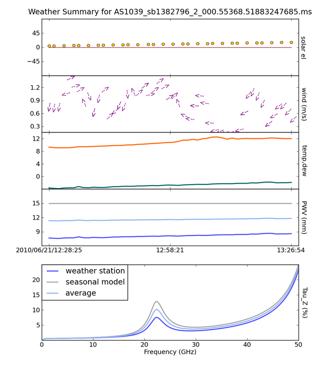
The weather information for a MS as plotted by the task {tt plotweather}.}
Determining opacity corrections for historical VLA data
For VLA data, zenith opacity can be measured at the frequency and during the time observations are made using a VLA tipping scan in the observe file. Historical tipping data are available here. Choose a year, and click Go to get a list of all tipping scans that have been made for that year.
If a tipping scan was made for your observation, then select the appropriate file. Go to the bottom of the page and click on the button that says Press here to continue. The results of the tipping scan will be displayed. Go to the section called ‘Overall Fit Summary’ to find the fit quality and the fitted zenith opacity in percent. If the zenith opacity is reported as 6%, then the actual zenith optical depth value is 0.060. Use this value in gencal as described above.
If there were no tipping scans made for your observation, then look for others made in the same band around the same time and weather conditions. If nothing is available here, then at K and Q bands you might consider using an average value (e.g. 6% in reasonable weather). See the VLA memo here for more on the atmospheric optical depth correction at the VLA, including plots of the seasonal variations.
Antenna-position corrections
When antennas are moved, residual errors in the geographical coordinates of the antenna will cause time-dependent delay errors in the correlated data. Normally, the observatory will solve for these offsets soon after the move and correct the correlator model, but sometimes science data is taken before the offsets are available, and thus the correction must be handled in post-processing. If the 3D position offsets for affected antennas are known, use gencal as follows:
gencal(vis='mydata.ms', caltable='antpos.cal', caltype='antpos', antenna='ea01',
       parameter=[0.01,0.02,0.005])
In this execution, the position offset for antenna ea01 is [1cm,2cm,0.5cm] in an Earth-centered right-handed coordinate system with the first axis on the prime meridian and third axis coincident with the Earth’s axis. Corrections for multiple antennas can be specified by listing all affected antennas and extending the parameter list with as many offset triples as needed.
In general, it is difficut to know what position offsets to use, of course. For the VLA, gencal will look up the required offests automatically, simply by omitting the antenna and parameter arguments:
gencal(vis='mydata.ms', caltable='antpos.cal', caltype='antpos')
For the historical VLA, the antenna position coordinate system was a local one translated from the Earth’s center and rotated to the VLA’s longitude. Use caltype=’antposvla’ to force this coordiate system when processing old VLA data.
The resulting calibration table should then be used in all subsequent processing the requires the specification of prior calibration.
Ionospheric corrections
WARNING: There are Known Issues regarding tec_map.
CASA 4.3 introduced initial support for on-axis ionospheric corrections, using time- and direction-dependent total electron content (TEC) information obtained from the internet. The correction includes the dispersive delay (\(\propto \nu^{-1}\)) delay and Faraday rotation (\(\propto \nu^{-2}\)) terms. These corrections are most relevant at observing frequencies less than \(\sim\) 5 GHz. When relevant, the ionosphere correction table should be generated at the beginning of a reduction along with other calibration priors (antenna position errors, gain curve, opacity, etc.), and carried through all subsequent calibration steps. Formally, the idea is that the ionospheric effects (as a function of time and on-axis direction) will be nominally accounted for by this calibration table, and thus not spuriously leak into gain and bandpass solves, etc. In practice, the quality of the ionospheric correction is limited by the relatively sparse sampling (in time and direction) of the available TEC information. Especially active ionospheric conditions may not be corrected very well. Also, direction-dependent (within the instantaneous field-of-view) ionosphere corrections are not yet supported. Various improvements are under study for future releases.
To generate the ionosphere correction table, first import a helper function from the casapy recipes repository:
from casatasks.private import tec_maps
Note that this only works for CASA 6.1.2 or later. For CASA 5, see here.
Then, generate a TEC surface image:
tec_maps.create(vis='mydata.ms',doplot=True,imname='iono')
This function obtains TEC information for the observing date and location from NASA’s CDDIS Archive of Space Geodesy Data, and generates a time-dependent CASA image containing this information. The string specified for imname is used as a prefix for two output images, with suffixes .IGS_TEC.im (the actual TEC image) and .IGS_RMS_TEC.im (a TEC error image). If imname is unspecified, the MS name (from vis) will be used as the prefix.
The quality of the retrieved TEC information for a specific date improves with time after the observing date as CDDIS’s ionospheric modelling improves, becoming optimal 1-2 weeks later. Both images can be viewed as a movie in the CASA task imview. If doplot=T, the above function will also produce a plot of the TEC as a function of time in a vertical direction over the observatory.
Finally, to generate the ionosphere correction caltable, pass the .IGS_TEC.im image into gencal, using caltype=’tecim’:
gencal(vis='mydata.ms',caltable='tec.cal',caltype='tecim',infile='iono.IGS_TEC.im')
This iterates through the dataset and samples the zenith angle-dependent projected line-of-sight TEC for all times in the observation, storing the result in a standard CASA caltable. Plotting this caltable will show how the TEC varies between observing directions for different fields and times, in particular how it changes as zenith angle changes, and including the nominal difference between science targets and calibrators.
This caltable should then be used as a prior in all subsequent calibration solves, and included in the final applycal.
A few warnings:
The TEC information obtained from the web is relatively poorly sampled in time and direction, and so will not always describe the details of the ionospheric corruption, especially during active periods.
For instrumental polarization calibration, it is recommended that an unpolarized calibrator be used; polarized calibrators may not yield as accurate a solution since the ionospheric corrections are not yet used properly in the source polarization portion of the polcal solve.
TEC corrections are only validated for use with VLA data. For data from other (low-frequency) telescopes, TEC corrections are experimental - please use at your own discretion.
Special thanks are due to Jason Kooi (UIowa) for his contributions to ionospheric corrections in CASA.
Switched-power (EVLA)
The EVLA is equipped with noise diodes that synchronously inject a nominally constant and known power contribution appropriate for tracking electronic gain changes with time resolution as short as 1 second. The total power in both the ON and OFF states of the noise diodes is continuously recorded, enabling a gain calibration derived from their difference (as a fraction of the mean total power), and scaled by a the approximately known contributed power (nominally in K). Including this calibration will render the data in units of (nominal) K, and also calibrate the data weights to units of inverse K2. To generate a switched-power calibration table for use in subsequent processing, run gencal as follows:
gencal(vis='myVLAdata.ms',caltable='VLAswitchedpower.cal',caltype='evlagain')
The resulting calibration table should then be used in all subsequent processing the requires the specification of prior calibration.
To ensure that the weight calibration by this table works correctly, it is important that the raw data weights are proprotional to integration time and channel bandwidth. This can be guaranteed by use of initweights as described above.
System Temperature (ALMA)
ALMA routinely measures \(T_{sys}\) while observing, and these measurements are used to reverse the online normalization of the correlation coefficients and render the data in units of nominal K. To generate a \(T_{sys}\) calibration table, run gencal as follows:
gencal(vis='myALMAdata.ms',caltable='ALMAtsys.cal',caltype='tsys')
The resulting calibration table should then be used in all subsequent processing the requires the specification of prior calibration.
Miscellaneous ad hoc corrections
The gencal task supports generating ad hoc amp, phase, and delay corrections via appropriate settings of the caltype parameter. Currently, such factors must be constant in time (gencal has no mechanism for specifying multiple timestamps for parameters), but sometimes such corrections can be useful. See the general gencal task documenation for more information on this type of correction.
Virtual Model Visibilities
The tasks that generate model visibilities (clean, tclean, ft, and setjy) can either (in most cases) save the data in a MODEL_DATA column inside of the MeasurementSet (MS) or it can save it in a virtual one. In the latter case the model visibilities are generated on demand when it is requested and the data necessary to generate that is stored (usually the Fourier transform of the model images or a component list). More detailed descriptions of the structure of an MS can be found on the CASA Fundamentals pages.
The tasks that can read and make use of the virtual model columns include calibration tasks, mstransform tasks (including uvsubtraction), plotms.
Advantages of virtual model column over the real one:
Speed of serving visibilities (in most cases because calculating models visibilities is faster than disk IO)
Disk space saving (a full size of the original data size is saved)
When not to use virtual model
When working with time-dependent models (e.g. ephemerides sources) within setjy; please use ephemerides source models only with usescratch=True
Model image size is a significant fraction of the visibility data size (e.g large cube from a small data set). Virtual model column serving might be slower than real one
When the user wants to edit the model physically via the table tool for e.g
When using an FTMachine that does not support virtual model saving when imaging (AWProjectFT for e.g)
Additional Information
When both a physical model column exists along with a virtual model, then the virtual model is the one that gets served by tasks that uses the visbuffer (e.g calibration tasks)
Use delmod* *task to manage your MODEL_DATA column and virtual model
If model data is written for a subset of the MS (say the user used field , spw and/or intent selection in tclean) then the model visibilities will be served properly for the subset in question the other part of the MS will have 1 served for parallel hand visibilities and 0 for crosshand visibilities. So be careful when doing calibration or uvsub after writing model visibilities only for a subset of the MS (this applies to using the physical scratch column MODEL_DATA too)
The virtual model info is written in the SOURCE table of the MS usually (and in the main table if the SOURCE table does not exist)
FTMachines (or imaging gridding mode) supporting virtual model data are:
GridFT: Standard gridder (including mutiterm and multi fields or cube),
WProjectFT: widefield wterm (including mutiterm and multi fields or cube),
MosaicFT: mosaic imaging (including mutiterm or cube),
ComponentLists
Solve for Calibration
The gaincal, bandpass, fringefit, polcal, and blcal tasks actually solve for the unknown calibration parameters from the visibility data obtained on calibrator sources, placing the results in a calibration table. They take as input an MS, and a number of parameters that specify any prior calibration tables to pre-apply before computing the solution, as well as parameters controlling the exact properties of the solving process.
We first discuss the parameters that are in common between many of the calibration tasks. Subsequent sub-sections will discuss the use of each of these solving task in more detail.
Common Calibration Solver Parameters
There are a number of parameters that are in common between the calibration solver tasks.
Input/output
The input MeasurementSet and output calibration table are controlled by the following parameters:
vis          =         ''   #Name of input visibility file
caltable     =         ''   #Name of output calibration table
The MS name is specified in vis. If it is highlighted red in the inputs then it does not exist, and the task will not execute. Check the name and path in this case.
The output table name is specified in caltable. Be sure to give a unique name to the output table, or be careful. If the table exists, then what happens next will depend on the task and the values of other parameters. The task may not execute giving a warning that the table already exists, or will go ahead and overwrite the solutions in that table, or append them. Be careful.
Data selection
Data selection is controlled by the following parameters:
field        =         ''   #field names or index of calibrators: ''==>all
spw          =         ''   #spectral window:channels: ''==>all
intent       =         ''   #Select observing intent
selectdata   =      False   #Other data selection parameters
Field and spectral window selection are so often used, that we have made these standard parameters, field and spw respectively. Additionally, intent is also included as a standard parameter to enable selection by the scan intents that were specified when the observations were set up and executed. They typically describe what was intended with a specific scan, i.e. a flux or phase calibration, a bandpass, a pointing, an observation of your target, or something else or a combination. The format for the scan intents of your observations are listed in the logger when you run listobs. Minimum matching with wildcards will work, like *BANDPASS*. This is especially useful when multiple intents are attached to scans. Finally, observation is an identifier to distinguish between different observing runs, mainly used for ALMA.
The selectdata parameter expands, revealing a range of other selection sub-parameters:
selectdata          =       True        #data selection parameters
     timerange      =         ''        #time range (blank for all)
     uvrange        =         ''        #uv range (blank for all)
     antenna        =         ''        #antenna/baselines (blank for all)
     scan           =         ''        #scan numbers (blank for all)
     correlation    =         ''        #correlations (blank for all)
     array          =         ''        #(sub)array numbers (blank for all)
     observation    =         ''        #Select by observation ID(s)
     msselect       =         ''        #MS selection (blank for all)
Note that if selectdata=False these parameters are not used when the task is executed, even if set non-trivially.
Among the most common selectdata=True parameters to use is uvrange, which can be used to exclude longer baselines if the calibrator is resolved, or short baselines if the calibrator contains extended flux not accounted for in the model. The rest of these parameters may be set according to information and values available in the listobs output. Note that all parameters are specified as strings, even if the values to be specified are numbers. See the section on MS Selection for more details on the powerful syntax available for selecting data.
Prior calibration
Calibration tables that have already been determined can be arranged for apply before solving for the new table using the following parameters:
docallib        =  False        #Use traditional cal apply parameters
     gaintable  =     []        #Gain calibration table(s) to apply on the fly
     gainfield  =     []        #Select a subset of calibrators from gaintable(s)
     interp     =     []        #Interpolation mode (in time) to use for each gaintable
     spwmap     =     []        #Spectral windows combinations to form for gaintable(s)
The docallib parameter is a toggle that can be used to select specification of prior calibration using the new “cal library” mechanism (docallib=True) which is described in greater detail here.
When docalib=False, the traditional CASA calibration apply sub-parameters will be used, as listed above.
gaintable
The gaintable parameter takes a string or list of strings giving the names of one or more calibration tables to arrange for application. For example:
gaintable = ['ngc5921.bcal','ngc5921.gcal']
specifies two tables, in this case bandpass and gain calibration tables respectively.
The gainfield, interp, and spwmap parameters key off gaintable, taking single values or lists, with an entries for each corresponding table in specified in gaintable. The caltables can be listed in gaintable in any order, without affecting the order in which they are applied to the data (for consistency, this is controlled internally according to the Measurement Equation framework). If non-trivial settings are required for only a subset of the tables listed in gaintable, it can be convenient to specify these tables first in gaintable, include their qualifying settings first in the other paramters, and omit specifications for those tables not needing qualification (sensible defaults will be used for these).
gainfield
The gainfield parameter specifies which field(s) from each respective gaintable to select for apply. This is a list, with each entry a string. The default for an entry means to use all in that table. For example, use
gaintable = ['ngc5921.bcal', 'ngc5921.gcal']
gainfield = [ '1331+305',    '1331+305,1445+099']
to specify selection of 1331+305 from ngc5921.bcal and fields 1331+305 and 1445+099 from ngc5921.gcal. Selection of this sort is only needed if avoiding other fields in these caltables is necessary. The field selection used here is the general MS Selection syntax.
In addition, gainfield supports a special value:
gainfield = [ 'nearest' ]
which selects the calibrator that is the spatially closest (in sky coordinates) to each of the selected MS fields specified in the field data selection parameter. Note that the nearest calibrator field is evaluated once per execution and is never dependent on time, spw or any other data meta-axis. This can be useful for running tasks with a number of different sources to be calibrated in a single run, and when this simple proximity notion is applicable. Note that the cal library mechanism provides increased flexibility in this area.
interp
The interp parameter chooses the interpolation scheme to be used when pre-applying the solution in the tables. Interpolation in both time and frequency (for channel-dependent calibrations) are supported. The choices are currently ‘nearest’ and ‘linear’ for time-dependent interpolation, and ‘nearest’, ‘linear’, ‘cubic’, and ‘spline’ for frequency-dependent interpolation. Frequency-dependent interpolation is only relevant for channel-dependent calibration tables (like bandpass) that are undersampled in frequency relative to the data.
‘nearest’ just picks the entry nearest in time or freq to the visibility in question
‘linear’ calibrates each datum with calibration phases and amplitudes linearly interpolated from neighboring values in time or frequency. In the case of phase, this mode will assume that phase never jumps more than 180 degrees between neighboring points, and so phase changes exceeding this between calibration solutions cannot be corrected for. Also, solutions will not be extrapolated arbitrarily in time or frequency for data before the first solution or after the last solution; such data will be calibrated using nearest to avoid unreasonable extrapolations.
‘cubic’ (frequency axis only) forms a 3rd-order polynomial that passes through the nearest 4 calibration samples (separately in phase and amplitude)
‘spline’ (frequency axis only) forms a cubic spline that passes through the nearest 4 calibration samples (separately in phase and amplitude)
For (unchannelized) time-dependent gaincal solutions, the time-dependent interp options can be appended with ‘PD’ to enable a “phase delay” correction per spw. For example: ‘nearestPD’ or ‘linearPD’. This will adjust the time-dependent phase by the ratio of the data frequency (centroid of the whole spw) and solution frequency (centroid of the spw channels selected when solved) and effect a time-dependent delay-like calibration over spws. This is most useful when distributing a single spw’s solution (or, e.g., as might be generated by combine=’spw’ in gaincal) to many data spws, and when the the residual spw phase being calibrated is purely non-dispersively delay-like, i.e., the residual spw phases for each antenna are instantaneously linear in frequency and imply phase=360n deg (n an integer) at zero frequency. This enables correcting rapidly-varying phases in high-frequency spws (such as caused by variable troposphere) using solutions derived from lower-frequency spws where the phase variations are smaller and the SNR typically greater, or for distributing solution phases derived in aggregate from a group of spws (using combine=’spw’) in a delay-like manner over the constituent spws. Note that use of the ‘PD’ suffix does not invoke a channel-dependent calibration within spws–the result still behaves as a gaincal solution, but will correct non-dispersive phase fluctuations in a manner that is effectively proportional to the centroid spw frequency. Also, the ‘PD’ algorithm has no choice but to assume that the available antenna solution phases start in the zeroth cycle, i.e., that, for each antenna, the relationship between the available spw phase and the target spw residual phases is linear and implies exactly zero phase (n=0) at zero frequency. For non-zero values of n, the implied phase at zero frequency is not zero, and the available spw solution phase is not in the zeroth cycle. In this case, the phases calculated for other spw frequencies will be offset by a (constant) fraction of a cycle equal to the fractional frequency difference between the solution and target spw frequencies. Thus, the ‘PD’ option cannot guarantee the instantaneous leveling of phase among spws at different frequencies; rather, it will reliably level time-dependent fluctuations in phases in each spw (when they are purely non-dispersive), and thereby possibly permit per-spw self-calibration on longer timescales to remove any remaining residuals, including any constant offsets described here. When using the ‘PD’ option, calibration results should be carefully examined.
The time-dependent interp options can also be appended with ‘perobs’ to enforce observation Id boundaries in the interpolation. Similarly, appending ‘perscan’ to the time-dependent interp options will enforce scan boundaries in the interpolation.
The frequency-dependent interp options can be appended with ‘flag’ to enforce channel-dependent flagging by flagged bandpass channels (i.e., ‘nearestflag’, ‘linearflag’, ‘cubicflag’, and ‘splineflag’, rather than to automatically fill such channels in with interpolation (which is the default).
For each gaintable, specify the interpolation style in quotes, with the frequency-dependent interpolation style specified after a comma, if relevant. For example:
gaintable = ['ngc5921.bcal',  'ngc5921.gcal']
gainfield = ['1331+305',      ['1331+305','1445+099'] ]
interp =    ['linear,spline', 'linear']
uses linear interpolation on the time axis for both cal tables, and a cubic spline for interpolation of the frequency axis in the bandpass table.
spwmap
The spwmap parameter is used to redistribute the calibration available in a caltable flexibly among spectral windows, thereby permitting correction of some spectral windows using calibration derived from others. The spwmap parameter takes a list or a list of lists of integers, with one list of integers for every caltable specified in gaintable. Each list is indexed by the MS spectral window ids, and the values indicate the calibration spectral windows to use for each MS spectral window. I.e., for each MS spw, i, the calibration spw j will be j=spwmap[i].
The default for spwmap (an empty list per gaintable) means that MS spectral windows will be calibrated by solutions identified with the same index in the calibration table (i.e., by themselves, typically). Explicit specification of the default would be spwmap=[0,1,2,3], for an MS with four spectral windows. Less trivially, for a caltable containing solutions derived from and labelled as spectral windows 0 and 1, these two cal spectral windows can be mapped to any of the MS spectral windows. E.g., (for a single gaintable):
spwmap=[0,1,1,0] #apply from cal spw=0 to MS spws 0,3 and from cal spw 1 to MS spws 1,2
For multiple gaintables, use a lists of lists (one spwmap list per gaintable), e.g.,
gaintable = ['ngc5921.bcal',  'ngc5921.gcal']
gainfield = ['1331+305',      ['1331+305','1445+099'] ]
interp =    ['linear,spline', 'linear']
spwmap =    [ [0,1,1,0],      [2,3,2,3] ]
which will use bandpass spws 0 and 1 for MS spws (0,3), and (1,2), respectively, and gain spws 2 and 3 for MS spws (0,2) and (1,3), respectively.
Any spectral window mapping is mechanically valid, including using specific calibration spectral windows for more than one different MS spectral window (as above) and using alternate calibration even for spectral windows for which calibration is nominally available, as long as the mapped calibration spectral windows have calibration solutions available in the caltable. If a mapped calibration spectral window is absent from the caltable (and not merely flagged), an exception will occur.
The scientific meaningfulness of a non-trivial spwmap specification is the responsibility of the user; no internal checks are performed to attempt the scientific validity of the mapping. Usually, spwmap is used to distribute calibration such as Tsys, which may be measured in a wide low-resolution spectral window, to narrow high-resolution spectral windows that fall within the wide one. It is also used to distribute calibration derived from a gaincal solve which was performed using combine=’spw’ (e.g., for increased SNR) to each of the spectral windows (and perhaps others) aggregated in the solve; in this case, it may be useful to consider using the ‘PD’ (“phase delay”) interpolation option described above, to account for the frequency ratios between each of the individual MS spectral windows and the aggregated calibration spectral window.
Absolute vs. Relative frequency in frequency-dependent interpolation
By default, frequency-dependent solutions are interpolated for application in absolute sky frequency units. Thus, it is usually necessary to obtain bandpass solutions that cover the frequencies of all spectral windows that must be corrected. In this context, it is mechanically valid to use spwmap to transfer a bandpass solution from a wide, low-resolution spectral window to a narrow, higher-resolution spectral window that falls within the wide one in sky frequency space. On the other hand, if adequate data for a bandpass solution is unavailable for a specific spectral window, e.g., due to contamination by line emission or absorption (such as HI), or because of flagging, bandpass solutions from other spectral windows (i.e., at different sky frequencies) can be applied using spwmap. In this case, it is also necessary to add ‘rel’ to the frequency interpolation string in the interp parameter, as this will force the interpolation to be calculated in relative frequency units. Specifically, the center frequency of the bandpass solution will be registered with the absolute center frequency of each of the MS spectral windows to which it is applied, thereby enabling relative frequency registration. The quality of such calibration transfer will depend, of course, on the uniformity of the hardware parameters and properties determining the bandpass shapes in the observing system–this is often appropriate over relatively narrow bandwidths in digital observing systems, as long as the setups are sufficiently similar (same sideband, same total spectral window bandwidth, etc., though note that the channelization need not be the same). Traditionally (e.g., at the VLA, for HI observations), bandpass solutions for this kind of calibration transfer have be solved by combining spectral windows on either side of the target spectral window (see the task documentation for bandpass for more information on solving with combine=’spw’).
For example, to apply a bandpass solution from spectral window 0 (in a bandpass table called ngc5921.bcal) to MS spectral windows 0,1,2,3 with linear interpolation calculated in relative frequency units (and with frequency-dependent flagging respected):
gaintable = ['ngc5921.bcal']
interp =    ['nearest,linearflagrel']
spwmap =    [ [0,0,0,0] ]
When selecting channels for a bandpass solution that will be applied using ‘rel’, it is important to recognize that the selected channels will be centered on each of the _absolute_ centers of the MS spectral windows to which it will be applied. An asymmetric channel selection for the bandpass solve will cause an undesirable shift in the relative registration on apply. Avoid this by using symmetrical channel selection (or none) for the bandpass solve.
Also note that if relative frequency interpolation is required but ‘rel’ is not used in interp, the interpolation mechanism currently assumes you want absolute frequency interpolation. If there is no overlap in absolute frequency, the result will be nearest (in channel) interpolation such that the calibration edge channel closest to the visibility data will be used to calibrate that data.
Finally, please note that relative frequency interpolation is not yet available via the cal library.
Parallactic angle
The parang parameter turns on the application of the antenna-based parallactic angle correction (P) in the Measurement Equation. This is necessary for polarization calibration and imaging, or for cases where the parallactic angles are different for geographically spaced antennas and it is desired that the ordinary calibration solves not absorb the inter-antenna parallactic angle phase. When dealing with only the parallel-hand data (e.g. RR, LL, XX, YY), and an unpolarized calibrator model for a co-located array (e.g. the VLA or ALMA), you can set parang=False and save some computational effort. Otherwise, set parang=True to apply this correction, especially if you are doing polarimetry.
Solving parameters
The parameters controlling common aspects of the solving process itself are:
solint              =      'inf'        #Solution interval: egs. 'inf', '60s' (see help)
combine             =     'scan'        #Data axes which to combine for solve (obs, scan,
                                        #spw, and/or field)
preavg              =       -1.0        #Pre-averaging interval (sec) (rarely needed)
refant              =         ''        #Reference antenna name(s)
minblperant         =          4        #Minimum baselines _per antenna_ required for solve
minsnr              =        3.0        #Reject solutions below this SNR
solnorm             =      False        #Normalize solution amplitudes post-solve.
corrdepflags        =      False        #Respect correlation-dependent flags
The time and frequency (if relevant) solution interval is specified in solint. Optionally a frequency interval for each solutglobal-task-list.ipynb#task_bandpassion can be added after a comma, e.g. solint=’60s,300Hz’. Time units are in seconds unless specified differently. Frequency units can be either ‘ch’ or ‘Hz’ and only make sense for bandpass or frequency dependent polarization calibration. On the time axis, the special value ‘inf’ specifies an infinite solution interval encompassing the entire dataset, while ‘int’ specifies a solution every integration. Omitting the frequency-dependent solution interval will yield per-sample solutions on this axis. You can use time quanta in the string, e.g. solint=’1min’ and solint=’60s’ both specify solution intervals of one minute. Note that ‘m’ is a unit of distance (meters); ‘min’ must be used to specify minutes. The solint parameter interacts with combine to determine whether the solutions cross scan, field, or other meta-data boundaries.
The parameter controlling the scope of each solution is combine. For the default, combine=’’, solutions will break at obs, scan, field, and spw boundaries. Specification of any of these in combine will extend the solutions over the specified boundaries (up to the solint). For example, combine=’spw’ will combine spectral windows together for solving, while combine=’scan’ will cross scans, and combine=’obs,scan’ will use data across different observation IDs and scans (usually, obs Ids consist of many scans, so it is not meaningful to combine obs Ids without also combining scans). Thus, to do scan-based solutions (single solution for each scan, per spw, field, etc.), set
solint = 'inf'
combine = ''
To obtain a single solution (per spw, per field) for an entire observation id (or the whole MS, if there is only one obsid), use:
solint = 'inf'
combine = 'scan'
You can specify multiple choices for combination by separating the axes with commas, e.g.:
combine = 'scan,spw'
Care should be exercised when using combine=’spw’ in cases where multiple groups of concurrent spectral windows are observed as a function of time. Currently, only one aggregate spectral window can be generated in a single calibration solve execution, and the meta-information for this spectral window is calculated from all selected MS spectral windows. To avoid incorrect calibration meta-information, each spectral window group should be calibrated independently (also without using append=True). Additional flexibility in this area will be supported in a future version.
The reference antenna is specified by the refant parameter. Ordinary MS Selection antenna selection syntax is used. Ideally, use of refant is useful to lock the solutions with time, effectively rotating (after solving) the phase of the gain solutions for all antennas such that the reference antennas phase remains constant at zero. In gaincal it is also possible to select a refantmode, either ‘flex’ or ‘strict’. A list of antennas can be provided to this parameter and, for refantmode=’flex’, if the first antenna is not present in the solutions (e.g., if it is flagged), the next antenna in the list will be used, etc. See the documentation for the rerefant task for more information. If the selected antenna drops out, the next antenna specified (or the next nearest antenna) will be substituted for ongoing continuity in time (at its current value) until the refant returns, usually at a new value (not zero), which will be kept fixed thenceforth. You can also run without a reference antenna, but in this case the solutions will formally float with time; in practice, the first antenna will be approximately constant near zero phase. It is usually prudent to select an antenna near the center of the array that is known to be particularly stable, as any gain jumps or wanders in the refant will be transferred to the other antenna solutions. Also, it is best to choose a reference antenna that never drops out, if possible.Setting a preavg time will let you average data over periods shorter than the solution interval first before solving on longer timescales. This is necessary only if the visibility data vary systematically within the solution interval in a manner independent of the solve-for factors (which are, by construction, considered constant within the solution interval), e.g., source linear polarization in polcal. Non-trivial use of preavg in such cases will avoid loss of SNR in the averaging within the solution interval.
The minimum signal-to-noise ratio allowed for an acceptable solution is specified in the minsnr parameter. Default is minsnr=3.
The minblperant parameter sets the minimum number of baselines to other antennas that must be preset for each antenna to be included in a solution. This enables control of the constraints that a solution will require for each antenna.
The solnorm parameter toggles on the option to normalize the solution after the solutions are obtained. The exact effect of this depends upon the type of solution (see gaincal, bandpass, and blcal). Not all tasks use this parameter.One should be aware when using solnorm that if this is done in the last stage of a chain of calibration, then the part of the calibration that is normalized away will be lost. It is best to use this in early stages (for example in a first bandpass calibration) so that later stages (such as final gain calibration) can absorb the lost normalization scaling. It is generally not strictly necessary to use solnorm=True at all, but it is sometimes helpful if you want to have a normalized bandpass for example.
The corrdepflags parameter controls how visibility vector flags are interpreted. If corrdepflags=False (the default), then when any one or more of the correlations in a single visibility vector is flagged (per spw, per baseline, per channel), it treats all available correlations in the single visibility vector as flagged, and therefore it is excluded from the calibration solve. This has been CASA’s traditional behavior (prior to CASA 5.7), in order to be conservative w.r.t. flags. If instead corrdepFlags=True (for CASA 5.7+), correlation-dependent flags will be respected exactly and precisely as set, such that any available unflagged correlations will be used in the solve for calibration factors. For the tasks currently supporting the corrdepflags parameter (gaincal, bandpass, fringefit, accor), this means any unflagged parallel-hand correlations will be used in solving, even if one or the other parallel-hand (or either of the cross-hands) is flagged. Note that the polcal task does not support corrdepflags since polarization calibration is generally more sensitive to correlation-dependence in the flagging in ways which may be ill-defined for partial flagging; this stricture may be relaxed in future for non-leakage solving modes. Most notably, this feature permits recovery and calibration of visibilities on baselines to antennas for which one polarization is entirely flagged, either because the antenna did not have that polarization at all (e.g., heterogeneous VLBI, where flagged visibilities are filled for missing correlations on single-polarization antennas), or one polarization was not working properly during the observation.
Appending calibration solutions to existing tables
The append parameter, if set to True, will append the solutions from this run to existing solutions in caltable. Of course, this only matters if the table already exists. If append=False and the specified caltable exists, it will overwrite it (if the caltable is not open in another process).
The append parameter should be used with care, especially when also using combine in non-trivial ways. E.g., calibration solves will currently refuse to append incongruent aggregate spectral windows (e.g., observations with more than one group of concurrent spectral windows) when using combine=’spw’. This limitation arises from difficulty determining the appropriate spectral window fan-out on apply, and will be relaxed in a future version.
Frequency and time labels for calibration solutions
Since calibration may be solved from aggregate ranges of frequency and time, it is interesting to consider how calibration solutions are labeled in frequency and time in caltables, based on the dataset from which they are solved, and also the relevance of this when applying the calibration to visibility data.
On the time axis, solutions are labeled with the unflagged centroid of the timestamps and baselines supplied to the solver, thereby permitting reasonably accurate time-dependent interpolation of solutions onto nearby data.
On the frequency axis, solutions are labeled with the channel-selected centroid frequencies, without regard to channelized flagging, at the frequency-axis granularity of the solutions. I.e., for per-spectral window and unchannelized gaincal solutions, this means the centroid frequency of the selected channels within each spectral window, and in the same frequency measures frame. For channelized bandpass solutions, this will be the centroid frequency of each (possibly partially aggregated) solution channel; if there is no frequency-axis solution interval, then the solution channel frequencies will be the same as the data channel frequencies, and in the same frequency measures frame. Note that the calibration table format demands that frequency labels are spectral-window specific and not time- or antenna-dependent; hence the possible time- and baseline-dependence of channel-dependent flagging cannot be accounted for in the frequency label information.
When combining spectral windows for calibration solves using combine=’spw’, the (selected) bandwidth-weighted centroid of all effectively-selected spectral windows will be used, and solutions will be identified with the lowest spectral window id in the effective spectral window selection. Note that it is the effective spectral window selection that matters, i.e., if user-specified scan or field or other non-spectral window selection effectively selects a subset of the spectral windows in a dataset (along with any explicit spw selection), only the net-selected spectral windows are used to calculate the net frequency label for the aggregate solution. Also, this net centroid frequency is calculated once per output spectral window (effectively for all solution intervals), even if the dataset is such that the constituent spectral windows are not available for all solutions. Thus, strictly speaking, the frequency labels will be less accurate for solution intervals containing only a subset of the global (selected) aggregate, and this may adversely affect the effective accuracy in the phase-delay (PD) calibration interpolation (described below). (Most raw datasets are not heterogeneous in this way.)
Note that combining multiple different groups of spectral windows with combine=’spw’ requires running the solving task separately for each group, and appending to the same caltable with append=True.
When appending solutions using multiple solving executions, the frequency label information for the net output solution spectral windows in the new execution must match what is already in the caltable, where there is overlap. If it does not, execution will be interrupted.
The solution frequency labels are relevant to the application of these solutions only if the specified interpolation mode or solution parameterization needs to care about it. E.g., for per-spectral window unchannelized gaincal solutions applied to the corresponding identical spectral windows in the visibility dataset (even if differently channel-selected), the solution frequency labels do not matter (the solutions are just directly applied)–unless the the time-axis interpolation includes the ‘PD’ option which will apply a scaling to the phase correction equal to the ratio of data frequency (whole spectral window centroid) and solution frequency. This ‘phase-delay’ interpolation mode enforces a delay-like adjustment to per-spectral window (not channelized) phases of the sort that is expected for non-dispersive tropospheric phase variations, and is much more interesting in the context of transferring phase calibration among spectral windows at different centroid freuqencies (even to different observing bands) using spwmap, including the case of a distributing a combined spectral window solution to the constituent spectral windows from which it was solved. (This interpolation mode is not likely to be very effective at observing frequencies and conditions where dispersive ionospheric phase effects are important.) Also, solutions that have a frequency-dependent parameterization such as from fringefit or gaincal with gaintype=’K’ (simple delays) require the centroid frequency label values recorded in the caltable to perform the net channelized solution phase calculation.
Bandpass solutions (from bandpass) will be non-trivially interpolated from the solution frequencies to the data frequencies in a conventional manner if the solutions were decimated in frequency when solved; if the solution frequencies exactly match the data frequencies, the solutions will just be directly applied.
In general, the centroid solution time and frequency labeling conventions described here are consistent with the assumption that calibration solutions are essentially constant during the time and frequency intervals within which they are solved, even if practically, there is some variation within these ranges. If this variation is significant, then the granularity at which the calibration is solved should be reconsidered, if possible, consistent with available SNR. Also, the available interpolation modes can be used to better track and compensate for gradients between solution samples. In all cases, solution granularity is constrained by a balance between available SNR and the systematic variation being sampled.
##Calibration solve task return dictionaries
The calibration solve tasks gaincal and bandpass return python dictionaries containing a variety of information about how they were executed and the properties of the calibration solutions obtained.
The following top-level dictionary keys contain execution parameter details:
‘apply_tables’ - the calibration tables specified through the task’s gaintable parameter, which will be applied on the fly
‘solve_table’ - the output calibration table
‘selectvis’ - a dictionary containing the data selection specified by the user. For each of the fields (‘antennas’, ‘field’, ‘intents’, ‘observation’, ‘scan’, and ‘spw’) there is a corresponding key that describes what has been selected. The value of all of these keys is an array of corresponding ids, or in the case of ‘intents’ an array of strings.
The ‘solvestats’ key contains a multi-layer python dictionary containing solution counting statistics on several meta-info axes and as a function of progress through the solving process. In each instance, the counting statistics are reported per-polarization: a 1- or 2-element list depending on the number of polarizations available in the dataset and the calibration type. To help diagnoses of where solution failures occur, the counts are reported for four different processing gates within the solving sequence:
‘expected’ - the total number of expected solution intervals from the selected data, without regard to flagging;
‘data_unflagged’ - the number of solution intervals surviving after accounting for data flagged (on disk, and by on-the-fly prior calibration application)
‘above_minblperant’ - the number of solution intervals surviving after applying minblperant as specified by the user (i.e., only those solution intervals with sufficient baselines per antenna)
‘above_minsnr’ - the number of solution intervals surviving after application of minsnr as specified by the user.
The counting at each of these cases is incremental in the order listed above, i.e., solutions failing an earlier gate cannot pass a later one.
At the top level of the solvestats dictionary, overall total solution interval counts are provided.
Also at the top level are keys referring to each spw (e.g., for spw id=0, ‘spw0’), within which the per-spectral window totals at each gate are recorded in the same manner.
Also for each spectral window, there is a distinct key for each antenna (e.g., for antenna id=0, ‘ant0’) that contains antenna-specific counts at each of the processing gates within that spectral window. For each antenna, there is also a key, ‘used_as_refant’ containing a count of how often the antenna was used as the refant.
This return dictionary is currently only supported for gaincal and bandpass. Deployment to other solve tasks (polcal, fringefit, etc.) is expected in future. For gaintype=’K’ solutions, note that the ‘above_minblperant’ and ‘above_minsnr’ gates are not meaningful as these thresholds are not explicitly applied for delay solutions (this will be improved in a future version).
Gain Calibration
In general, gain calibration includes solving for time- and frequency-dependent multiplicative calibration factors, usually in an antenna-based manner. CASA supports a range of options.
Note that polarization calibration is described in detail in a different section.
Frequency-dependent calibration: bandpass
Frequency-dependent calibration is discussed in the general task documentaion for bandpass.
Gain calibration: gaincal
Gain calibration is discussed in the general task documentation for gaincal.
Flux density scale calibration: fluxscale
Flux density scale calibration is discussed in the general task documentation for fluxscale.
Baseline-based (non-closing) calibration: blcal
Non-closing baseline-based calibration is disussed in the general task documentation for blcal.
Polarization Calibration
Instrumental polarization calibration is necessary because the polarizing hardware in the receiving system will, in general, be impure and non-orthogonal at a level of at least a few percent. These instrumental polarization errors are antenna-based and generally assumed constant with time, but the algebra of their effects is more complicated than the simple ~scalar multiplicative gain calibration. Also, the net gain calibration renders the data in an arbitrary cross-hand phase frame that must also be calibrated. The polcal task provides support for solving for instrumental polarization (poltype=’Df’ and similar) and cross-hand phase (‘Xf’). Here we separately describe the heuristics of solving for instrumental polarization for the circular and linear feed bases.
Polarization Calibration in the Circular Basis
Fundamentally, with good ordinary gain and bandpass calibration already in hand, good polarization calibration must deliver both the instrumental polarization and position angle calibration. An unpolarized source can deliver only the first of these, but does not require parallactic angle coverage. A polarized source can only also deliver the position angle calibration if its polarization position angle is known a priori. Sources that are polarized, but with unknown polarization degree and angle, must always be observed with sufficient parallactic angle coverage (which enables solving for the source polarization), where “sufficient” is determined by SNR and the details of the solving mode.
These principles are stated assuming the instrumental polarization solution is solved using the “linear approximation” where cross-terms in more than a single product of the instrumental or source polarizations are ignored in the Measurement Equation. A more general non-linearized solution, with sufficient SNR, may enable some relaxation of the requirements indicated here, and modes supporting such an approach are currently under development.
For instrumental polarization calibration, there are 3 types of calibrator choice, listed in the following table:
Cal Polarization |
PA Coverage |
Poln Model? |
poltype |
Result |
|---|---|---|---|---|
Zero |
any |
Q=U=0 |
‘Df’ |
D-terms only |
Unknown |
2+ scans |
ignored |
‘Df+QU’ |
D-terms and Q,U |
Known, non-zero |
2+ scans |
Set Q,U |
‘Df+X’ |
D-terms and Pos Angle |
Note that the parallactic angle ranges spanned by the scans in the modes that require this should be large enough to give good separation between the components of the solution. In practice, 60 degrees is a good target.
Each of these solutions should be followed with a ‘Xf’ solution on a source with known polarization position angle (and correct fractional Q+iU in the model).
The polcal task will solve for the ‘Df’ or ‘Xf’ terms using the model visibilities that are in the model attached to the MS. Calibration of the parallel hands must have already been obtained using gaincal and bandpass in order to align the amplitude and phase over time and frequency. This calibration must be supplied through the gaintable parameters, but any caltables to be used in polcal must agree (e.g. have been derived from) the data in the DATA column and the FT of the model. Thus, for example, one would not use the caltable produced by fluxscale as the rescaled amplitudes would no longer agree with the contents of the model.
Be careful when using resolved calibrators for polarization calibration. A particular problem is if the structure in Q and U is offset from that in I. Use of a point model, or a resolved model for I but point models for Q and U, can lead to errors in the ‘Xf’ calibration. Use of a uvrange will help here. The use of a full-Stokes model with the correct polarization is the only way to ensure a correct calibration if these offsets are large.
A note on channelized polarization calibration
When your data has more than one channel per spectral window, it is important to note that the calibrator polarization estimate currently assumes the source polarization signal is coherent across each spectral window. In this case, it is important to be sure there is no large cross-hand delay still present in your data. Unless the online system has accounted for cross-hand delays (typically intended, but not always achieved), the gain and bandpass calibration will only correct for parallel-hand delay residuals since the two polarizations are referenced independently. Good gain and bandpass calibration will typically leave a single cross-hand delay (and phase) residual from the reference antenna. Plots of cross-hand phases as a function of frequency for a strongly polarized source (i.e., that dominates the instrumental polarization) will show the cross-hand delay as a phase slope with frequency. This slope will be the same magnitude on all baselines, but with different sign in the two cross-hand correlations. This cross-hand delay can be estimated using the gaintype=’KCROSS’ mode of gaincal (in this case, using the strongly polarized source 3C286):
gaincal(vis='polcal_20080224.cband.all.ms',
        caltable='polcal.xdelcal',
        field='3C286',
        solint='inf',
        combine='scan',
        refant='VA15',
        smodel=[1.0,0.11,0.0,0.0],
        gaintype='KCROSS',
        gaintable=['polcal.gcal','polcal.bcal'])
Note that smodel is used to specify that 3C286 is polarized; it is not important to specify this polarization stokes parameters correctly in scale, as only the delay will be solved for (not any absolute position angle or amplitude scaling). The resulting solution should be carried forward and applied along with the gain (.gcal) and bandpass (.bcal) solutions in subsequent polarization calibration steps.
Circular Basis Example
In the following example, we have a MS called polcal_20080224.cband.all.ms for which we already have bandpass, gain and cross-hand delay solutions. An instrumental polarization calibrator with unknown linear polarization has been observed. We solve for the instrumental polarization and source linear polarization with polcal using poltype=’Df+QU’ as follows:
polcal(vis= 'polcal_20080224.cband.all.ms',
       caltable='polcal.pcal',
       field='2202+422',
       solint='inf',
       combine='scan',
       preavg=300.0,
       refant='VA15',
       poltype='Df+QU',
       gaintable=['polcal.gcal','polcal.bcal','polcal.xdelcal])
This run of polcal assumes that the model stored in the MS for 2202+422 is the one that was used to obtain the net gain calibration stored in polcal.gcal (i.e., we have not substituted a fluxscale result, which would create an inconsistent scale).
Alternatively, if we have an instrumental polarization calibrator that we know is unpolarized, we run polcal with poltype=’Df’:
polcal(vis='polcal_20080224.cband.all.ms',
       caltable='polcal.pcal',
       field='0319+415',
       refant='VA15',
       poltype='Df',
       gaintable=['polcal.gcal','polcal.bcal','polcal.xdelcal])
In general, if there is more than one calibrator suitable for instrumental polarization calibration, it is useful to obtain a solution from each of them, and compare results. The instrumental polarization should not vary with field, of course. Note that it is not yet possible to effectively use combine=’field’ for instrumental polarization calibration solves with polcal, unless the prior models for all fields are set to the correct apparent linear polarization for each.
Having obtained the instrumental polarization calibration, we solve for the cross-hand phase using the flux density calibrator (for which the instrinsic linear polarization is known):
polcal(vis='polcal_20080224.cband.all.ms',
       caltable= 'polcal.polx',
       field='0137+331',
       refant='VA15',
       poltype='Xf',
       smodel=[1.0,-0.0348,-0.0217,0.0],   #the fractional Stokes for 0137+331 (3C48)
       gaintable=['polcal.gcal','polcal.bcal','polcal.xdelcal','polcal.pcal'])
Note that the correct fractional polarization has been specified for 0137+331. It is not necessary to use the correct absolute total and linearly polarized flux densities here, since the Xf calibration is entirely phase-like.
Polarization Calibration in the Linear Feed Basis
CASA now supports instrumental polarization calibration for the linear feed basis at a level that is practical for the general user. Some details remain to be implemented with full flexibility, and much of what follows will be streamlined in future releases.
Calibrating the instrumental polarization for the linear feed basis is somewhat more complicated than the circular feed basis because the polarization effects (source and instrument) appear in all four correlations at first or zeroth order (whereas for circular feeds, the polarization information only enters the parallel hand correlations at second order). As a result, e.g., the time-dependent gain calibration will be distorted by any non-zero source polarization, and some degree of iteration will be required to isolate the gain calibration if the source polarization is not initially known. These complications can actually be used to advantage in solving for the instrumental calibration; in can be shown, for example, that a significantly linearly polarized calibrator enables a better instrumental polarization solution than an unpolarized calibrator.
In the following example, we show the processing steps for calibrating the instrumental polarization using a strongly (>5%) polarized point-source calibrator (which is also the time-dependent gain calibrator) that has been observed over a range of parallactic angle (a single scan is not sufficient). We assume that we have calibrated the gain, bandpass, and cross-hand delay as described elsewhere, and that the gain calibration was obtained assuming the calibrator was unpolarized.
Linear Basis Example
First, we import some utility functions from the CASA recipes area:
from recipes.almapolhelpers import *
Our MS in this example is called polcal_linfeed.ms. We begin by assuming we already have a bandpass calibration result (obtained by conventional means) stored in polcal.bcal. We first solve for a time-dependent gain solution on the instrumental polarization calibrator, which we expect to be significantly polarized, but for which we do not yet have a polarization model:
gaincal(vis='polcal_linfeed.ms',
        caltable='polcal.gcal',
        field='1',                 #the instrumental polarization calibrator
        solint='int',
        smodel=[1,0,0,0],          #assume zero polarization
        gaintype='G',
        gaintable=['polcal.bcal'],
        parang=T)                  #so source poln properly rotated
Since the gain calibrator was assumed unpolarized, the time-dependent gain solutions contain information about the source polarization. This can be seen by plotting the amp vs. time for this cal table using poln=’/’. The antenna-based polarization amplitude ratios will reveal the sinusoidal (in parallactic angle) function of the source polarization. Run the utility method qufromgain to extract the apparent source polarization estimates for each spw:
qu=qufromgain('polcal.gcal')
The source polarization reported for all spws should be reasonably consistent. This estimate is not as good as can be obtained from the cross-hands (see below) since it relies on the gain amplitude polarization ratio being stable which may not be precisely true. However, this estimate will be useful in resolving an ambiguity that occurs in the cross-hand estimates.
Next we estimate both the XY-phase offset and source polarization from the cross-hands. The XY-phase offset is a spectral phase-only bandpass relating the X and Y systems of the reference antenna. If the XY-phase is solved for in a channel-dependent manner (as below), it is strictly not necessary to have solved for the cross-hand delay as described above, but it does not hurt, as it allows reasonably coherent channel averages for data examination (we assume below that we have obtained the cross-hand delay solution at this stage). The source polarization occurs in the cross-hands as a sinusoidal function of parallactic angle that is common to both cross-hands on all baselines (for a point-source). If the XY-phase bandpass is uniformly zero, then the source linear polarization function will occur entirely in the real part of the cross-hand visibilities. Non-zero XY-phase has the effect of rotating the source linear polarization signature partially into the imaginary part, where circular (and instrumental) polarization occur (cf. the circular feed basis where the cross-hand phase merely rotates the position angle of linear polarization). The following gaincal solve averages all baselines together and first solves for a channelized XY-phase (the slope of the source polarization function in the complex plane in each channel), then corrects the slope and solves for a channel-averaged source polarization. This calibration is obtained using gaintype=’XYf+QU’ in gaincal:
gaincal(vis='polcal_linfeed.ms',
        caltable='polcal.xy0amb',  #possibly with 180deg ambiguity
        field='1',                 #the calibrator
        solint='inf',
        combine='scan',
        preavg=200.0,              #minimal parang change
        smodel=[1,0,1,0],          #non-zero U assumed
        gaintype='XYf+QU',
        gaintable=['polcal.gcal','polcal.bcal','polcal.xdelcal])  #all prior calibration
Note that we imply non-zero Stokes U in smodel; this is to enforce the assumption of non-zero source polarization signature in the cross-hands in the ratio of data and model. This solve will report the center-channel XY-phase and apparent Q,U for each spw. The Q,U results should be recognizable in comparison to that reported by qufromgain above. However, since the XY-phase has a 180 degree ambiguity (you can rotate the source polarization signature to lie entirely in the visibility real part by rotating clockwise or counter-clockwise), some or all spw Q,U estimates may have the wrong sign. We correct this using the xyamb utility method, using the qu obtained from qufromgain above (which is not ambiguous):
S=xyamb(xy='polcal.xy0amb',qu=qu,xyout='polcal.xy0')
The python variable S now contains the mean source model (Stokes I =1; fractional Q,U; V=0) that can be used in a revision of the gain calibration and instrumental polarization calibration.
Next we revise the gain calibration using the full polarization source model:
gaincal(vis='polcal_linfeed.ms',
        caltable='polcal.gcal1',
        field='1',
        solint='int',
        smodel=S,                  #obtained from xyamb
        gaintype='G',
        gaintable=['polcal.bcal'],
        parang=T)                  #so source poln properly rotated
Note that parang=T so that the supplied source linear polarization is properly rotated in the parallel-hand visibility model. This new gain solution can be plotted with poln=’/’ as above to show that the source polarization is no longer distorting it. Also, if qufromgain is run on this new gain table, the reported source polarization should be statistically indistinguishable from zero.
Finally, we can now solve for the instrumental polarization:
polcal(vis= 'polcal_linfeed.ms',
       caltable='polcal.dcal',
       field='1',
       solint='inf',
       combine='scan',
       preavg=200,
       poltype='Dflls',      #freq-dep LLS solver
       refant='',            #no reference antenna
       smodel=S,
       gaintable=['polcal.gcal1','polcal.bcal','polcal.xdelcal','polcal.xy0'])
Note that no reference antenna is used since this solve will produce an absolute instrumental polarization solution that is registered to the assumed source polarization (S) and prior calibrations. Applying a refant (referring all instrumental polarization terms to a reference antennas X feed, which would then be assumed perfect) would, in fact, discard valid information about the imperfections in the reference antennas X feed. (Had we used an unpolarized calibrator, we would not have a valid xy-phase solution, nor would we have had access to the absolute instrumental polarization solution demonstrated here.)
A few points:
Since the gain, bandpass, and XY-phase calibrations were obtained prior to the instrumental polarization solution and maybe distorted by it, it is generally desirable to re-solve for them using this instrumental polarization solution as a prior calibration. In effect, this means iterating the sequence of calibration steps using all of the best of the available information at each stage, including the source polarization (and parang=T). This is a generalization of traditional self-calibration.
If the source linear polarization fraction and position angle is known a priori, the processing steps outlined above can be amended to use that source polarization assertion in the gain and instrumental calibration solves from the start. The qufromgain method is then not needed (but can be used to verify assumptions), the gaincal(…,gaintype=XYf+QU,…) should not be altered (parallactic angle coverage is still required!), and the xyamb run should use the a priori polarization for qu. If there is likely to be a large systematic offset in the mean feed position angle, iteration of the gain, bandpass, and instrumental polarization terms is required to properly isolate the calibration effects.
Note that the above process does not explicitly include a position angle calibration. In effect, the estimated source polarization sets the mean feed position angle as the reference position angle, and this is usually within a degree or so of optimal for linear feeds. If your mean X feed position angle is not 0 degrees, and your MS does not account for the offset in its FEED subtable, be careful in your interpretation of the final position angle. Currently, the circular feed-specific position angle calibration modes of polcal(…,poltype=’Xf’,…) will not properly handle the linear feed basis; this will be fixed in a future release.
Water Vapor Radiometers
The task wvrgcal generates a gain table based on Water Vapor Radiometer (WVR) data and is used for ALMA data reduction. Briefly, the task enables a Bayesian approach to calculating the coefficients that convert the outputs of the ALMA 183 GHz water-vapor radiometers (mounted on each antenna) into estimates of path fluctuations which can then be used to correct the observed interferometric visibilities.
The task is based on the wvrgcal software and the underlying libair and libbnmin libraries which were developed by Bojan Nikolic at the University of Cambridge as part of EU FP6 ALMA Enhancement program. The algorithmic core of wvrgcal is described in three ALMA memos (number 587 [1], 588 [2], and 593 [3] ).
The original wvrgcal software version 1.2 (described in the above memos) provided a stand-alone shell executable as the user interface. The implementation made heavy use of the Boost C++ libraries. Over the years since the ALMA inauguration, the software was extended with several features such as flagging and the application of offsets tables (wvrgcal v2.1). Up to CASA 6.6.4, the executable was embedded into CASA via a system call from the CASA task interface. In 2024, wvrgcal v3.0 was created by removing all dependencies on Boost and turning the software into a proper CASA tool (named “wvr”) and the executable into a tool method (named “gcal”). The task now calls this tool and the stand-alone executable is no longer provided. This greatly improved the runtime performance of wvrgcal. There was no change to the task interface which continues to follow closely the interface of the orignal shell executable at the same time staying within the CASA task parameter conventions.
In ALMA data, the WVR measurements belonging to a given observation are contained in the ASDM for that observation. After conversion to an MS using importasdm, the WVR information can be found in a separate spectral window (typically spectral window 0). The wvrgcal task identifies the SPW autonomously, but it can also be specified via the parameter wvrspw (see below). The specified spectral window(s) must be present in the MS for wvrgcal to work. This is not to be mixed up with the list of spectral windows for which solutions should be calculated and which can be specified with the parameter spw. Note that wvrgcal will calculate a correction only for the scans with the words ON_SOURCE, SIGNAL, or REFERENCE in the scan intent. The various features of wvrgcal are then controlled by a number of task parameters (see the list above). They have default values which will work for ALMA data. An example for a typical wvrgcal call can be found in the ALMA CASA guide for the NGC 3256 analysis:
wvrgcal(vis='uid___A002_X1d54a1_X5.ms',
     caltable='cal-wvr-uid___A002_X1d54a1_X5.W',
     toffset=-1,
     segsource=True, tie=["Titan,1037-295,NGC3256"], statsource="1037-295",
     wvrspw=[4],
     spw=[17,19,21,23])
Here, vis is the name of input visibility file which as mentioned above also contains the WVR data and caltable is the name of the output gain calibration table. WVR data is typically in spectral window 0, but in the example above, the data are contained in spectral window 4. Although wvrgcal should automatically identify this SPW, it is explicitly specified with the wvrspw parameter in the above example. The toffset parameter is the known time offset in seconds between the WVR measurements and the visibility integrations for which they are valid. For ALMA, this offset is presently -1 s (which is also the default value).
The parameter segsource (segregate source) controls whether separate coefficients are calculated for each source. The default value True is the recommended one for ALMA. When segsource is True, the subparameter tie is available. It permits the formation of groups of sources for which common coefficients are calculated as well as possible. The tie parameter ensures best possible phase transfer between a group of sources. In general it is recommended to tie together all of the sources in a single Science Goal (in ALMA speak) and their phase calibrator(s). The recommended maximum angular distance up to which two sources can be tied is 15 degrees. The parameter statsource controls for which sources statistics are calculated and displayed in the logger. This has no influence on the generated calibration table.
Via the parameter spw, one can control for which of the input spectral windows wvrgcal will calculate phase corrections and store them in the output calibration table. By default, solutions for all spectral windows are written except for the ones containing WVR data. The wvrgcal task respects the flags in the Main and ANTENNA table of the MS. The parameter mingoodfrac lets the user set a requirement on the minimum fraction of good measurements for accepting the WVR data from an antenna. If antennas are flagged, their WVR solution is interpolated from the three nearest neighboring antennas. This process can be controlled with the new parameters maxdistm and minnumants. The former sets the maximum distance an antenna used for interpolation may have from the flagged one. And minnumants sets how many near antennas there have to be for interpolation to take place. For more details on the WVR Phase correction, see also the the ALMA Memo “Quality Control of WVR Phase Correction Based on Differences Between WVR Channels” by B. Nikolic, R. C. Bolton & J. S. Richer [4] , see also ALMA memo 593 [3].
Statistical parameters shown in the logger output of wvrgcal
The wvrgcal task writes out a variety of information to the logger, including various statistical measures of the performance. This allows the user to judge whether WVR correction is appropriate for the MS, to check whether any antennas have problematic WVR values, and to examine the predicted performance of the WVR correction when applied. For each set of correction coefficients which are calculated (the number of coefficient sets are controlled by the parameters nsol, segsource and tie), the wvrgcal output to the logger first of all shows the time sample, the individual temperatures of each of the four WVR channels, and the elevation of the source in question at that time. For each of these coefficient sets, it then gives the evidence of the bayesian parameter estimation, the calculated precipitable water vapor (PWV) and its error in mm, and the correction coefficients found for each WVR channel (dTdL).
The output then shows the statistical information about the observation. First of all it gives the start and end times for the parts of the observation used to calculate these statistics (controlled by segsource). It then shows a break down for each of the antennas in the data set. This gives the antenna name and number; whether or not it has a WVR (column WVR); whether or not it has been flagged (column FLAG); the RMS of the path length variation with time towards that antenna (column RMS); and the discrepancy between the RMS path length calculated separately for different WVR channels (column Disc.). These values permit the user to see if an individual WVR appears to have been suffering from problems during the observation, and to flag the radiometer of that antenna using wvrflag if necessary. This discrepancy value, Disc., can in addition be used as a simple diagnostic tool to evaluate whether or not the WVR correction caltable created by wvrgcal should be applied. In the event of the WVR observations being contaminated by strong cloud emission in the atmosphere, the attempt by wvrgcal to fit the water vapor line may not be successful, and applying the produced calibration table can in extreme cases reduce the quality of the data. However, these weather conditions may be identified by a high value in the discrepancy column produced when running wvrgcal.
Discrepancy values of greater than a 1000 microns usually indicate strong cloud contamination of the WVR data, and the output calibration table should probably not be applied. If the values are between 100 and 1000 microns, then the user should manually examine the phases before and after applying the caltable to decide if WVR correction is appropriate. ALMA has developed an additional routine to at least partially remove the cloud component from the WVR data before calculating phase corrections (“remove_cloud”) which produces a table of offsets to be applied to the WVR data before fitting the water line via the wvrgcal parameter offsetstable. This feature has been available since CASA 4.7 and is now also used in the standard ALMA QA procedures, when needed.
After the antenna-by-antenna statistics, the output then displays some estimates of the performance of the wvrgcal correction. These are the thermal contribution from the water vapor to the path fluctuations per antenna (in microns), the largest path fluctuation found on a baseline (in microns), and the expected error on the path length calculated for each baseline due to the error in the coefficients (in microns).
Antenna position calculation
The information about antenna pointing direction is by default taken from the POINTING table. Should this table not be present for some reason, the user can instead switch to determining the antenna positions from the phase directions in the FIELD table (under the assumption that all antennas were pointing ideally). The switch is performed by setting the parameter usefieldtab to True.
Spectral window selection
By default, wvrgcal puts solutions for all spectral windows of the MS into the output calibration table. Since usually only those spectral windows are of interest in which the science target and the calibrators were observed, it is not necessary to store solutions for other spectral windows. The spectral windows for which solutions are stored can be selected with the parameter spw, e.g. spw = [17,19,21,23] will make wvrgcal write only solutions for spectral windows 17, 19, 21, and 23. With respect to the input WVR spectral windows, wvrgcal will by default regard all windows with 4 channels as WVR data. In typical ALMA data there is only one such spectral window in each ASDM. In any case, the input WVR spectral window(s) can be selected with the optional parameter wvrspw. The syntax is the same as for the parameter spw above.
Bibliography
Examine/Edit Cal Tables
How to plot, list, and adjust calibration tables
Information on examination and manipulation of calibration tables can be found in the task documentation for plotms, listcal, calstat, smoothcal, and browsetable.
Apply Calibration
How to apply calibration to generate data for imaging
Please see the task documentation for applycal for details on application of calibration.