Open in Colab: https://colab.research.google.com/github/casangi/casadocs/blob/v6.3.0/docs/notebooks/usingcasa.ipynb
Using CASA
See the CASA API for information on configuration options prior to startup.
Starting CASA
CASA packages installed through pip may be imported in to the standard Python environment on the host machine. For example:
(casa6) $ python

Python 3.6.9 (default, Nov 7 2019, 10:44:02)
[[GCC 8.3.0] on linux]
Type "help", "copyright", "credits" or "license" for more information.
>>> import casatasks
>>> help(casatasks)
The ~/.casa/config.py file will be read and processed when the casatasks package is imported.
The full installation of CASA includes an IPython environment which is executed like an application. Any desired command line arguments may be included. For example:
$ ./casa6/bin/casa --logfile MyTestRun.txt --nogui
The ~/.casa/config.py file will be read and processed as the casa application executes, with the supplied command line arguments (logfile and nogui) added on top.
This environment is based upon IPython. CASA uses IPython because it provides nice command completion, comandline editing and function invocation without parenthesis. The fact that the CASA application environment is IPython based means that users can also use the IPython magic commands like %run. Users are encouraged to explore the options available with IPython, but this is outside the scope of this document. CASA only supports configuration using config.py. Some of these configuration
variable in config.py are used to configure IPython at startup time. CASA configures IPython to supply parentheses when they are omitted. For example, when sin 3 is executed IPython supplies the missing parens and invokes sin(3). CASA also turns off any output that the paren expansion would normally generate.
Users may wish to set shortcuts, links, aliases or add bin/casa to their envrionment PATH. See the documentation for your operating system.
Running User Scripts
CASA 6: modular version
The modular version of CASA behaves like a standard Python package and user scripts should include the relevant modules as they would any other python module (i.e. numpy). Executing external user scripts with modular CASA is just like any other python application. Note we recommend running in a Python venv, see the installation instructions for more information.
$ (casa6) python myscript.py param1 param2
CASA 6: all-inclusive version
Since the full CASA installation from a tar file includes its own python environment that is (typically) not called directly, alternative methods of feeding in user scripts are necessary. There are three main standard Python ways of executing external user scripts in the full installation of CASA:
-c startup parameter (see configuration instructions)
exec(open(“./filename”).read()) within the CASA Python environment
add your script to startup.py in the ~/.casa directory
In addition, an “execfile” python shortcut has been added to the full installation of CASA 6 for backwards compatibility with ALMA scriptForPI.py restore scripts. This allows running scripts with the following command:
execfile ‘filename.py’ within the CASA Python environment
The execfile command in CASA 6 has been tested and found to work in the same way as in (Python 2 based) CASA 5 with the exception that (1) the treatment of global variables has changed in Python 3, (2) only direct arguments should be used (i.e., listobs(vis=’name.ms’)), and (3) the command default(‘taskname’) no longer works with execfile (but note that direct arguments always invoke the defaults anyway). While casashell tasks (tasks run in the CASA shell environment) could be treated as scriptable in the Python 2.7/CASA 5 version of execfile, in Python 3/CASA 6 this behavior is not supported. Python replacements for execfile exist [i.e., “%run -i” or “exec(open(read…”] which provide some scripting capabilities for casashell commands, though these Python alternatives are not tested in any internal CASA regression tests.
Regarding the treatment of global variables: for execfile calls within a script which itself is run via execfile, it is necessary to add globals() as the second argument to those execfile calls in order for the nested script to know about the global variables of the calling script. For example, within a script ‘mainscript.py’, calls to another script ‘myscript.py’ should be written as follows: execfile(‘myscript.py’, globals()) .
Logging
Detailed description of the CASA logger
Logging your session
The output from CASA commands is sent to the file casa-YYYYMMDD-HHMMSS.log in your local directory, where YYYYMMDD-HHMMSS are the UT date and time when CASA was started up. New starts of CASA create new log files.
The CASA Logger GUI window under Linux. Note that under MacOSX a stripped down logger will instead appear as a Console.
The output contained in casa-YYYYMMDD-HHMMSS.log is also displayed in a separate window using the casalogger. Generally, the logger window will be brought up when CASA is started. If you do not want the logger GUI to appear, then start casa using the –nologger option,
casa --nologger
which will run CASA in the terminal window. See Starting CASA for more startup options.
ALERT: Due to problems with Qt , the GUI qtcasalogger is a different version on MacOSX and uses the Mac Console. This still has the important capabilities such as showing the messages and cut/paste. The following description is for the Linux version and thus should mostly be disregarded on OSX. On the Mac, you treat this as just another console window and use the usual mouse and hot-key actions to do what is needed.
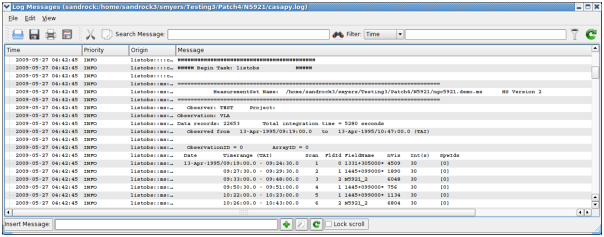
The CASA logger window for Linux is shown in the figure above. The main feature is the display area for the log text, which is divided into columns. The columns are:
Time — the time that the message was generated. Note that this will be in local computer time (usually UT) for casa generated messages, and may be different for user generated messages;
Priority — the Priority Level (see below) of the message;
Origin — where within CASA the message came from. This is in the format Task::Tool::Method (one or more of the fields may be missing depending upon the message);
Message — the actual text.
The CASA Logger GUI window under Linux. Note that under MacOSX a stripped down logger will instead appear as a Console.
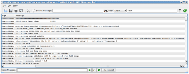
Using the casalogger Filter facility. The log output can be sorted by Priority, Time, Origin, and Message. In this example we are filtering by Origin using ‘clean’, and it now shows all the log output from the clean task.
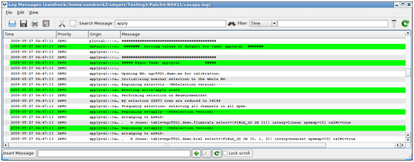
The casalogger GUI has a range of features, which include:
Search — search messages by entering text in the Search window and clicking the search icon. The search currently just matches the exact text you type anywhere in the message.
Filter — a filter to sort by message priority, time, task/tool of origin, and message contents. Enter text in the Filter window and click the filter icon to the right of the window. Use the pull-down at the left of the Filter window to choose what to filter. The matching is for the exact text currently (no regular expressions).
View — show and hide columns (Time, Priority, Origin, Message) by checking boxes under the View menu pull-down. You can also change the font here.
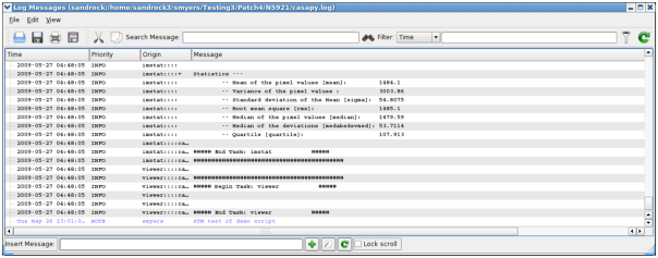
Insert Message — insert additional comments as “notes” in the log. Enter the text into the “I*nsert Message*” box at the bottom of the logger, and click on the Add (+) button, or choose to enter a longer message. The entered message will appear with a priority of “NOTE” with the Origin as your username.
Copy — left-click on a row, or click-drag a range of rows, or click at the start and shift click at the end to select. Use the Copy button or Edit menu Copy to put the selected rows into the clipboard. You can then (usually) paste this where you wish.
Open — There is an Open function in the File menu, and an Open button, that will allow you to load old casalogger files.
Alert: Messages added through Insert Message will currently not be inserted into the correct (or user controllable) order into the log. Copy does not work routinely in the current version. It is recommended to open the casa-YYYYMMDD-HHMMSS.log file in a text editor, to grab text.
CASA Logger - Insert facility: The log output can be augmented by adding notes or comments during the reduction. The file should then be saved to disk to retain these changes.
Other operations are also possible from the menu or buttons. Mouse “flyover” displays a tooltip describing the operation of buttons.
It is possible to change the name of the logging file. By default it is ‘casa-YYYYMMDD-HHMMSS.log’. But starting CASA with the option *–logfile *will redirect the output of the logger to the file ‘otherfile.log’ (see also Page on “Starting CASA”).
casa --logfile otherfile.log
The log file can also be changed during a CASA session. Typing:
casalog.setlogfile('otherfile.log')
will redirect the output to the ‘otherfile.log*’* file. However, the logger GUI will still be monitoring the previous ‘casa-YYYYMMDD-HHMMSS.log’ file. To change it to the new file, go on File - Open and select the new log file, in our case ‘otherfile.log*’*.
Startup options for the logger
One can specify logger options at the startup of CASA on the command line:
casa <logger options>
The options are described in “Starting CASA”. For example, to inhibit the a GUI and send the logging messages to your terminal, do
casa --nologger --log2term
while
casa --logfile mynewlogfile.log
will start CASA with logger messages going to the file mynewlogfile.log. For no log file at all, use:
casa --nologfile
Setting priority levels in the logger
Logger messages are assigned a Priority Level when generated within CASA. The current levels of Priority are:
SEVERE — errors;
WARN — warnings;
INFO — basic information every user should be aware of or has requested;
INFO1 — information possibly helpful to the user;
INFO2 — details for advanced users;
INFO3 — continued details;
INFO4 — lowest level of non-debugging information;
DEBUGGING — most “important” debugging messages;
DEBUG1 — more details;
DEBUG2 — lowest level of debugging messages.
The “debugging” levels are intended for the developers use.
Inside the Toolkit:
The casalog tool can be used to control the logging. In particular, the casalog.filter method sets the priority threshold. This tool can also be used to change the output log file, and to post messages into the logger.
There is a threshold for which these messages are written to the casa-YYYYMMDD-HHMMSS.log file and are thus visible in the logger. By default, only messages at level INFO and above are logged. The user can change the threshold using the casalog.filter method. This takes a single string argument of the level for the threshold. The level sets the lowest priority that will be generated, and all messages of this level or higher will go into the casa-YYYYMMDD-HHMMSS.log file.
Some examples:
casalog.filter('INFO')           #the default
casalog.filter('INFO2')          #should satisfy even advanced users
casalog.filter('INFO4')          #all INFOx messages
casalog.filter('DEBUG2')         #all messages including debuggingcasalog.
WARNING: Setting the threshold to DEBUG2 will put lots of messages in the log!
Error Handling with CASA tasks
Irrecoverable errors in tasks produce exceptions in all CASA tasks. Different standard Python types of exceptions are thrown depending on the type of error, including RuntimeError, OSError, ValueError, or AssertionError (in particular when there is an error validating the input parameters). This behavior applies to all CASA tasks and has been made consistent across all tasks beginning with CASA 6.2/5.8. For a list of CASA tasks see the API section.
When using CASA tasks in their modular version (from the casatasks module), the exceptions are thrown as in normal Python functions, and can be used to handle errors in the data reduction workflow in user scripts, pipelines, etc. In earlier versions of CASA this was not consistent; see the changes section below for more details on earlier versions of CASA.
Let us see an example script that in CASA 6 produces an exception in the task split:
from casatasks import split
try:
    split(vis='uid___A002_X30a93d_X43e_small.ms', outputvis='foo.ms', datacolumn='corrected', spw='0')
except RuntimeError as exc:
    print(' * Got exception: {}'.format(exc))
The task fails and produces an exception because the requested data column is not present in the MeasurementSet. The print statement (shown here as a trivial way of handling the error, just for illustration) will print the following message:
* Got exception: Desired column (CORRECTED_DATA) not found in the input MS (/casadata/uid___A002_X30a93d_X43e_small.ms).
The following messages are also produced in the CASA log:
INFO    split::::casa   ##########################################
INFO    split::::casa   ##### Begin Task: split              #####
INFO    split::::casa   split( vis='uid___A002_X30a93d_X43e_small.ms', outputvis='foo.ms', keepmms=True, field='', spw='0', scan='', antenna='', correlation='', timerange='', intent='', array='', uvrange='', observation='', feed='', datacolumn='corrected', keepflags=True, width=1, timebin='0s', combine='' )
INFO    MSTransformManager::parseMsSpecParams   Input file name is uid___A002_X30a93d_X43e_small.ms
INFO    MSTransformManager::parseMsSpecParams   Data column is CORRECTED
INFO    MSTransformManager::parseMsSpecParams   Output file name is foo.ms
INFO    MSTransformManager::parseDataSelParams  spw selection is 0
WARN    MSTransformManager::checkDataColumnsToFill  CORRECTED_DATA column requested but not available in input MS
INFO    MSTransformManager::initDataSelectionParams Selected SPWs Ids are Axis Lengths: [1, 4]  (NB: Matrix in Row/Column order)
INFO    MSTransformManager::initDataSelectionParams+    [0, 0, 3, 1]
INFO    MSTransformManager::open    Select data
INFO    MSTransformManager::createOutputMSStructure Create output MS structure
SEVERE  split::::casa   Task split raised an exception of class RuntimeError with the following message: Desired column (CORRECTED_DATA) not found in the input MS (/casadata/uid___A002_X30a93d_X43e_small.ms).
INFO    split::::casa   Task split complete. Start time: 2020-11-02 14:33:58.083124 End time: 2020-11-02 14:33:58.262353
INFO    split::::casa   ##### End Task: split                #####
INFO    split::::casa   ##########################################
CASA 6 - casashell (monolithic) version of tasks
When starting CASA in its full installation variant, using the bin/casa command, a version of the CASA tasks meant for interactive use in the CASA IPython prompt is automatically imported. These interactive or casashell versions of the CASA tasks (see casashell) support, for example, the inp/go commands. The behavior of these casashell tasks in terms of error handling is intentionally different from the behavior of the modular version of the tasks, as explained
below. Note that this doesn’t imply that the modular tasks behavior cannot be obtained when using the full installation. The modular version of a task can be imported by simply importing the task explicitly from casatasks.
The casashell versions of the tasks do not throw exceptions. Instead, they return False if an exception occurs within the task. The exception traceback is printed to the CASA log, but the execution of the task finishes without throwing the exception. The casashell infrastructure captures the exceptions that occur inside a task and turn any exception into a return value False. For example, if we use the same split command from the previous section in the CASA prompt, which fails because a
non-existent data column is requested, the split call will return False and the log will show the following messages:
CASA <1>: split(vis='uid___A002_X30a93d_X43e_small.ms', outputvis='foo.ms', datacolumn='corrected', spw='0')
INFO    split::::casa   ##########################################
INFO    split::::casa   ##### Begin Task: split              #####
INFO    split::::casa   split( vis='uid___A002_X30a93d_X43e_small.ms', outputvis='foo.ms', keepmms=True, field='', spw='0', scan='', antenna='', correlation='', timerange='', intent='', array='', uvrange='', observation='', feed='', datacolumn='corrected', keepflags=True, width=1, timebin='0s', combine='' )
INFO    MSTransformManager::parseMsSpecParams   Input file name is uid___A002_X30a93d_X43e_small.ms
INFO    MSTransformManager::parseMsSpecParams   Data column is CORRECTED
INFO    MSTransformManager::parseMsSpecParams   Output file name is foo.ms
INFO    MSTransformManager::parseDataSelParams  spw selection is 0
WARN    MSTransformManager::checkDataColumnsToFill  CORRECTED_DATA column requested but not available in input MS
INFO    MSTransformManager::initDataSelectionParams Selected SPWs Ids are Axis Lengths: [1, 4]  (NB: Matrix in Row/Column order)
INFO    MSTransformManager::initDataSelectionParams+    [0, 0, 3, 1]
INFO    MSTransformManager::open    Select data
INFO    MSTransformManager::createOutputMSStructure Create output MS structure
SEVERE  split::::casa   Task split raised an exception of class RuntimeError with the following message: Desired column (CORRECTED_DATA) not found in the input MS (/casadata/uid___A002_X30a93d_X43e_small.ms).
INFO    split::::casa   Task split complete. Start time: 2020-11-02 18:27:59.105823 End time: 2020-11-02 18:27:59.316335
INFO    split::::casa   ##### End Task: split                #####
INFO    split::::casa   ##########################################
SEVERE  split::::casa   Exception Reported: Error in split: Desired column (CORRECTED_DATA) not found in the input MS (/casadata/uid___A002_X30a93d_X43e_small.ms).
INFO    split::::casa   Traceback (most recent call last):
INFO    split::::casa+    File "/scratch/casa-6.2.0-36/lib/py/lib/python3.6/site-packages/casashell/private/split.py", line 723, in __call__
INFO    split::::casa+      _return_result_ = _split_t( _invocation_parameters['vis'],_invocation_parameters['outputvis'],_invocation_parameters['keepmms'],_invocation_parameters['field'],_invocation_parameters['spw'],_invocation_parameters['scan'],_invocation_parameters['antenna'],_invocation_parameters['correlation'],_invocation_parameters['timerange'],_invocation_parameters['intent'],_invocation_parameters['array'],_invocation_parameters['uvrange'],_invocation_parameters['observation'],_invocation_parameters['feed'],_invocation_parameters['datacolumn'],_invocation_parameters['keepflags'],_invocation_parameters['width'],_invocation_parameters['timebin'],_invocation_parameters['combine'] )
INFO    split::::casa+    File "/scratch/casa-6.2.0-36/lib/py/lib/python3.6/site-packages/casatasks/split.py", line 258, in __call__
INFO    split::::casa+      task_result = _split_t( _pc.document['vis'], _pc.document['outputvis'], _pc.document['keepmms'], _pc.document['field'], _pc.document['spw'], _pc.document['scan'], _pc.document['antenna'], _pc.document['correlation'], _pc.document['timerange'], _pc.document['intent'], _pc.document['array'], _pc.document['uvrange'], _pc.document['observation'], _pc.document['feed'], _pc.document['datacolumn'], _pc.document['keepflags'], _pc.document['width'], _pc.document['timebin'], _pc.document['combine'] )
INFO    split::::casa+    File "/scratch/casa-6.2.0-36/lib/py/lib/python3.6/site-packages/casatasks/private/task_split.py", line 163, in split
INFO    split::::casa+      mtlocal.open()
INFO    split::::casa+    File "/scratch/casa-6.2.0-36/lib/py/lib/python3.6/site-packages/casatools/mstransformer.py", line 43, in open
INFO    split::::casa+      return self._swigobj.open()
INFO    split::::casa+    File "/scratch/casa-6.2.0-36/lib/py/lib/python3.6/site-packages/casatools/__casac__/mstransformer.py", line 176, in open
INFO    split::::casa+      return _mstransformer.mstransformer_open(self)
INFO    split::::casa+  RuntimeError: Desired column (CORRECTED_DATA) not found in the input MS (/casadata/uid___A002_X30a93d_X43e_small.ms).
Out[1]: False
(in this example listing we show what would be printed to the terminal when the CASA log messages are printed to the terminal, using the --log2term command line option).
In CASA 5, by default tasks never threw exceptions. See an earlier version of CASA Docs for details.
Standardized behavior since CASA 6.2
The behavior of tasks with respect to errors, exceptions, and return values in case of error has been standardized since CASA 6.2. In CASA 6.x, this standardization applies only to CASA tasks when imported from casatasks. The casashell versions that come with casashell (CASA IPython prompt) keep the same behavior: they never throw exceptions and instead return False in case of a serious error (exception in the task). This is ensured by the casashell infrastructure (casashell task wrappers)
that will never let an exception out.
The changes introduced are:
All tasks throw exceptions as normal Python functions (the one or more top level try/except blocks that would trap all exceptions in 1/3+ of tasks have been removed or replaced in favor of finally blocks that clean up tools, etc. resources, see documentation on Python clean-up actions and the finally clause.
Exception types are more specific, using different Python built-in exceptions and avoiding the overly generic ‘Exception’ type as much as possible.
The message when there is an exception in a task is the same for all tasks, is printed to the CASA log and reads, for example, like this: “Task <mstransform> raised an exception of class <RuntimeError> with the following message: Desired column (CORRECTED_DATA) not found in the input MS (/casadata/uid___X02_X3d737_X1_01_small.ms)”
The same behavior when there are errors in HISTORY updates is ensured across all CASA tasks: produce a warning message but don’t change the task return/exceptions.
The situation before/after these changes can be summarized as follows:
In CASA releases earlier than 6.2/5.8, some tasks would raise exceptions, but other tasks would never raise exceptions. Instead, they would trap any exceptions raised in the task and return different values representing unsuccessful execution, such as False, None, or {}. To know whether exceptions were raised or something else returned (and what particular something else was returned), one would need to look into the task code, as this was undocumented behavior and there was no clear pattern to explain the different behavior of different tasks.
Beginning in CASA 6.2, all CASA tasks raise exceptions in the event of an unrecoverable error, as they would be raised by normal Python functions. Client code using CASA tasks can assume all tasks raise exceptions in case of error and devise a consistent error handling approach when using CASA tasks.
The following list summarizes the tasks which will raise exceptions after CASA 6.2/5.8 but did not raise exceptions in earlier versions of CASA:
from casatasks: clearcal, clearstat, cvel2, delmod, fixplanets, fixvis, flagdata, hanningsmooth, imhead, importasdm, importatca, importgmrt, importmiriad, importuvfits, imregrid, imsmooth, initweights, listcal, listfits, listhistory, listobs, listpartition, listvis, mstransform, nrobeamaverage, partition, plotants, sdpolaverage, sdtimeaverage, setjy, specfit, split, spxfit, uvsub, vishead
from casaplotms: plotms
The impact on scripts that use these tasks is that errors will now be more visible, with an exception raised rather than a probably silent and ambiguous False or None or {} return. Note that scripts that do not import tasks explicitly from casatasks are implicitly using the casashell version of the tasks. These scripts would not see any behavior changes, as in their case the casashell tasks never throw exceptions. In scripts that use tasks from casatasks and were not checking
the return value of tasks (for example for a False or {} value), potential failures in tasks would remain potentially hidden in the code flow, before CASA 6.2/5.8 (and maybe unnoticed). From CASA 6.2/5.8 onward, a failure in a task will raise an exception. Scripts can implement error handling to react to exceptions from tasks by using the try clause of Python.
Information Collection
To better understand real-world usage patterns, quality and reliability, CASA collects runtime telemetry and crash reports from users and sends periodic reports back to NRAO. This information is anonymous with no personal identifiable information (PII) or science data included.
Telemetry
Telemetry records task usage activity (task name, start time, end time) during CASA runs. Periodically, these reports will be batched together and sent to NRAO.
You can disable telemetry by adding the following line in ~/.casa/config.py
telemetry_enabled = False
Telemetry adds log files in the “rcdir” (e.g., ~/.casa) directory and submits the data at CASA startup after a predefined interval. This can be configured in the ~/.casa/config.py file by setting telemetry_submit_interval to a desired value in seconds. The default value is 1 week.
The log file cache directory can be changed by setting “telemetry_log_directory” in ~/.casa/config.py. “telemetry_log_directory” must be an absolute path.
Maximum telemetry log usage can be set with “telemetry_log_limit” (in kilobytes). CASA will check for the logfile size periodically and disable Telemetry when the limit is reached. The check interval can be set with “telemetry_log_size_interval” (seconds).
Summary of all available options in .casa/config.py:
telemetry_log_directory: /tmp
telemetry_log_limit: 1650
telemetry_log_size_interval: 30
telemetry_submit_interval: 20
Crash Reporter
Crash reports are triggered whenever a CASA task terminates abnormally (e.g., unhandled C++ exception, segfault, etc.). The crash reports include:
program call stack
filesystem mount information
CASA log
memory information
operating system version
CPU information
You can disable crash reports by adding the following line in ~/.casa/config.py
crashreporter_enabled = False
Hardware Requirements
Recommended CASA computing environments
The recommended Hardware requirements are provided here as part of the CASA webpages.
Amazon Web Services
Overview of how to use CASA on Amazon Web Services
An introduction to Amazon Web Services
In this chapter you will learn how to create an account within AWS, select appropriate resources for a problem, launch those resources, perform any desired processing, return or store resulting products, and finally to release the reserved resources back to Amazon.

Amazon Web Services Introduction
Amazon Web Services (AWS) is a collection of physical assets and software tools for using ad hoc computing resources (aka Cloud Computing) within Amazon. The combination of a wide range of processing hardware, network speeds, storage media and tools allows users to create virtual computing platforms tailored to specific problem sizes with discrete durations.
In simplest terms, AWS allows users to create workstations or medium sized clusters of computers (ranging from 10’s to a few 1000 nodes) that are essentially identical to the kind of physical workstation or small cluster they might have at their home institution without the overhead of upfront capital expense, space, power or cooling. The full range of offerings from Amazon goes well beyond that simple conceptual model but many, if not most, are not directly applicable to radio astronomy data processing.
The target audience for this document is the astronomer who wishes to run their computations more quickly, would like to know if AWS can help accomplish that goal, and what possibilities and limitations AWS brings.
Applicability to NRAO Data Processing
NRAO data products, particularly those from the Atacama Large Millimeter Array (ALMA) and the Jansky Very Large Array (JVLA), are of sufficient volume (100s to 1000s of GBytes) and compute complexity to require processing capabilities ranging from high end workstations to small clusters of servers. Additionally advanced imaging algorithms typically benefit from more system memory than is likely available on standard desktops.
AWS can facilitate the transfer of data among researchers through high speed networks or shared storage. Large scale projects which can be decomposed along some axis (e.g. by observation, field, frequency, etc) can be processed concurrently across 10s, 100s or even 1000s of compute instances.
Document Outline
This document set attempts to walk users through the necessary steps to create an account within AWS, select appropriate resources for their problem, launch those resources, perform any desired processing, return or store resulting products to the user, and finally to release the reserved resources back to Amazon. The last step is a critical aspect to the financial viability of computing within AWS. Later sections will cover the potential financial benefit and possible pitfalls of utilizing AWS resources.
Requesting Assistance
Given the unique nature of AWS resources, please direct any questions or comments to nrao-aws@nrao.edu rather than to CASA or Helpdesk personnel.
User Account Setup
Creating and setting up a user account on AWS
Overview
To facilitate fine grain control of AWS resources, Amazon supplies two distinct account types. A Root user account (Account Root User) and Identity and Access Management Users (IAM Users). Learn more.
These accounts are distinct from regular Linux accounts that may exist on a compute instance.
Account Root User
Click here and follow the steps to set up an Amazon Web Services account.
Signing up for an AWS account automatically creates a Root user account with total control over the account. The credit card used during sign-up will be billed for all usage by the Account Root User and the Account’s IAM Users.
In general, the Root user account should only be used for changing account wide settings, e.g. creating or removing IAM users, changing AWS support plan or closing the account. An IAM User account should be used when requesting resources. Following this model allows for finer grain control over the type and scale of resources a specific user can request, and can limit the risk from unexpected expenses or accidental global changes to the account.
IAM Users
Getting Started with IAM Users
View Amazon’s AWS Documentation
The Root Account User can create IAM Users. These IAM Users may have more limited permissions or they may have Administrators permissions. It is recommended the Root Account User first create an IAM User in the Administrators group. That IAM User can then login and perform essentially all administrative operations, including adding more IAM Users.
IAM users can be given different levels of permissions for requesting AWS resources. Perimissions can be mapped to a User via membership in an IAM group or by having an IAM Role mapped to the User. More information on creating and utilizing IAM groups and IAM Roles can be found here
Other Resources - How to Sign into AWS as an IAM User : View Amazon’s AWS Documentation - Best practices for using IAM Users : View Amazon’s AWS Documentation
Linux Users
View Amazon’s AWS Documentation
IAM Users typically have the ability to start Instances, a virtual machine running Linux on AWS hardware. While starting the instance, an ssh key is specified. That key can be used to ssh into the running instance.
Adding Additional Linux Users : View Amazon’s AWS Documentation
Amazon Machine Images
An Amazon Machine Image (AMI) provides the information required to launch an instance, which is a virtual server in the cloud
Overview
An AMI is an object that encapsulates a base OS image (e.g., Red Hat Enterprise Linux, CentOS, Debian), any 3rd party software packages (e.g., CASA, SciPy) and any OS level run time modifications (e.g., accounts, data, working directories). Since an AMI is a discrete object, it can be mapped onto differing hardware instances to provide a consistent work environment independent of the instance’s number of processors, available memory, or total storage space.
The NRAO provides a set of pre-made images based on the standard Amazon image, which include specific release versions of CASA and Python and AWS’s command line interface (CLI) and application programming interface (API). The appropriate AMI can be used to start an image with operating system and software ready to run CASA.
Finding an NRAO AMI
You can search for NRAO AMIs using the console.
From the navigation bar in the upper right, change your region to be “US West (Oregon)”
Open the AWS Console and click on “EC2 Dashboard”.
Click on “AMIs” to bring up the interface for selecting AMIs.
The AMI selection interface by default displays only AMIs “Owned by me”. Change it to “Public Images”.
Narrow this long list to only NRAO images.
Click in the box to the right of the magnifying glass.
A menu listing “Resource Attributes” will pop up below the box you clicked on. Ignore it and type “NRAO” in the box and press the Enter key.
The list of AMIs has been narrowed to NRAO AMIs only.
New NRAO AMIs will be released periodically.
Using an AMI
Click the box next to the AMI you want. Click Launch. The Instances section of this document covers starting instances.
Geographic Locales
AWS has the concept of Regions and Zones in which Instances, EBS volumes, S3 buckets, and other resources are run. So an S3 bucket may be in region us-west-2 and not directly accessible if another IAM User is currently using us-east-1. However, a user may select the region they run in. And users may also duplicate some resouces across regions if access latency is the concern. To find the latency from your computer to all the AWS regions, try the cloudping tool: http://www.cloudping.info.
AMIs are Region-specific
An AWS AMI User can only use AMIs stored in its region. However, copying an AMI to another region is straightforward. The copy gets a new AMI-ID, so it effectively becomes a new AMI; the original AMI-ID is appended to the new AMI’s “Description”. The new AMI always starts out private and may need to be made public. (It takes about 15 minutes after making an AMI public for it to show up in a search.) In every other way, it is a duplicate of the original.
To make the image public, select the AMI and from the “Actions” menu and pick “Modify Image Permissions”. As in this image select “Public” and click Save.
Storage
AWS provides four basic forms of storage that vary by speed, proximity to their associated instance (which impacts latency/performance), and price.
The sections below describe storage in roughly the order of proximity to the instance. To first order each, subsequent type decreases in both performance and cost with Glacier being the slowest and cheapest. EBS may be the most commonly used.
Instance Store
Instance stores are solid state drives physically attached to the hardware the instance is running on that are available only on certain instance types. (Use of instance stores is beyond the scope of this document, although more information is available at this AWS page.) It is indirectly the most expensive form of storage since instance types with instance store capacity also include extra processor cores and memory. Cost effectiveness is a function of whether the extra cores and memory are utilized. Instance stores do not use redundant hardware. Instance stores cannot preserve their data after their instance stops.
Elastic Block Storage (EBS)
EBS is connected to instances via high speed networks and is stored on redundant hardware. EBS persists independently after a compute instance terminates (although it may be set to terminate instead). EBS storage can be allocated during the creation of an instance, or it may be created separately and attached to an existing instance. It may be detached from one instance and re-attached to another, which is potentially useful where the processing requirements for one stage of processing (e.g., calibration and flagging) are substantially different from a later stage (e.g., imaging).
Simple Storage Service (S3)
S3 storage is an object level store (rather than a block level store) designed for medium to long-term storage. Most software applications like CASA do not interact directly with S3 storage. Instead, one of the AWS Interfaces to S3 is used. Typically, S3 is used to temporarily store data before moving it to an EBS or Instance store volume for processing. Or it is used as long term storage for final products. As of this writing, S3 storage costs range from $150 - $360 TByte/year, depending on whether data is flagged as infrequent access. Longer term storage utilizes Glacier storage.
Glacier
Glacier is the lowest cost AWS storage. Data within S3 can be flagged for migration to glacier where it is copied to tape. As of this writing, Glacier storage costs roughly $86 TByte/year. Retrival from Glacier takes ~4 hours.
Instances
An instance is effectively a single computer composed of an OS, processors, memory, base storage and optional additional data storage
Instance Types
Amazon has predefined over 40 instance types. These fall into classes defined roughly by processing power, which are further subdivided by total memory and base storage.
Click here to see a list of all Linux instance types with their number of virtual CPUs (vCPU), total memory in GBytes of RAM, and the type of storage utilized by the instance type.
Note the “vCPU” is actually a hyperthread, so 2 “vCPU” equal one core, e.g. m4.xlarge has 2 cores. (These prices are for on-demand instances.)
Starting Instances
CASA requires >=4GB/core. Storage can be EBS. Because AWS has hyperthreading turned on, each “vCPU” is one hyperthread and therefore 2 vCPUs essentially equal 1 physical core. Some experimentation may be required to optimize the instance type if many instances are to be used. This can have a very significant impact on total run time and cost. The 4GB per physical core rule should be sufficient to get started.
Choosing a Payment Option: On-demand vs. Spot
Choosing an on-demand instance (the default) guarantees you the use of that instance (barring hardware failure).
There is also a Spot Price market; click here to read about it. The price of an instance fluctuates over time as a function of demand. AWS fills spot requests starting at the highest bid and working down to the lowest, the bid price paid by all spot users is the bid price reached when all resources were exhausted. When you request a spot instance you submit a bid for those resources. If that bid exceeds the current spot price, then the spot instance will launch and continue to run as long as the spot price remains below the bid. Typically, the spot price is much less than the on-demand price, so bidding the on-demand price typically permits an instance to run its job to completion. During the time it runs, it is billed only at the running spot price, not the bid, so the savings can be considerable. If the spot price rises above your bid your instance will be terminated. Be warned, if demand is excessive for that particular instance type and you bid 2x or more of the on-demand price you run the risk of the spot price rising to that level. Over bidding the demand price is most useful for very long running jobs where it’s considered acceptable to pay more for brief periods while minimizing the risk that the instance will be terminated due to a low bid.
For example, the on-demand price for a m4.xlarge instance is $0.239 per hour. For the past 3 months, the mean spot price has been $0.0341 (maximum $0.0515 per hour). A 10-hour run of 100 instances would have cost $239 for on-demand and $34 for spot instances. That assumes adding 100 instances to the spot market will not affect the spot price much, which is a reasonable assumption. However, adding 500 instances will certainly raise the spot price.
It’s possible to bid up to 10 times the on-demand price.
There are other ways to purchase AWS instances, but only on-demand and spot instances appear of interest to running CASA. See purchasing options.
Monitoring
A critical aspect to the financial viability of computing within AWS
Instance Monitoring
After a job finishes on an instance, that instance and storage are still running and generating charges to the AWS Account Root User. Instances and storage known to not be needed can of course be shut down. To check whether an instance is in use or not, a quick check can be made using the console: Click Instances, check the box next to your instance, and select the “Monitoring” tab. CPU Utilization is shown. But to be really sure, login to the instance and check if your job is finished. If so, you can transfer data off the root volume as needed and terminate the instance.
For more information see: http://docs.aws.amazon.com/AmazonCloudWatch/latest/DeveloperGuide/US_SingleMetricPerInstance.html#d0e6752
Storage Monitoring (EBS)
After the instance terminates, the instance ID and data volume names will continue to show up for several minutes. This can be used to find EBS volumes that were attached to the instance. If the user does not want their data to remain on EBS, i.e., to transfer their EBS volume to another instance or save it for later, then terminating the volume at that time makes sense. Although, the user might want to preserve the data by copying it to S3 or downloading it to a local storage device and then terminate the EBS volume.
Storage Monitoring (S3)
If you have data in S3 you may wish to leave it there. If you wish to move it to your local storage device, click the cube in the upper left of the console, then choose S3. Unfortunately the console is clumsy for transferring data. Reading through the Interfaces section of this chapter (and the relevant links), specifically on the use of the AWS CLI, is therefore recommended. Once the user is done with the previously allocated AWS resources, the user can release the reserved resources back to Amazon.
Interfaces
Amazon has multiple interface methods for interacting with resources.
The AWS console is a web interface used to control AWS resources. For users launching isolated instances and querying status, this is likely the simplest and most commonly used interface.
The CLI is the command line interface to AWS. This software, installed on your local computer, can be used to launch and control AWS resources. This interface is most useful for repeated tasks and simple automation
The python SDK interface is beyond the scope of this document, but more information can be found here. The python interface is most useful for complex automation frameworks and includes a REST-ful interface to all AWS resources.
Example Using CASA
Tutorial of CASA on AWS
Overview of Using CASA on AWS
Amazon Web Services (AWS) allows researchers to use instances for NRAO data processing. This section presents readying an Instance to process a data set with CASA. The CASA tutorial will be used as a demonstration of running CASA on AWS.
Choose an Instance
The tutorial does not require an instance with a lot of CPU and RAM. Per the hardware requirements page section on memory: 500MB per core is adequate. An m4.xlarge is more than adequat and costs $0.24/hour. It has 2 cores and 16 GB RAM. A smaller instance such as m4.large would probably work as well, except it has 1 core and could not run things in parallel.
Get Ready to Start an Instance
Follow the directions on the AMI page to locate an NRAO AMI. Select the AMI, and from the Actions menu, choose Launch. Select the m4.xlarge image type, which, as mentioned above, should be adequate for the tutorial at 2 cores and 8 GB/core. After that, we often press the “Review and Launch” button to skip to the end of the process. However, we need to add some storage first.
Start an Instance with Some Extra Storage Space
Select “4. Add Storage” at the top. You can see the root volume is by default 8 GB. For the tutorial, we might get by with 8 GB, but enlarging the root volume will remove any doubt. Change 8 to 1024 (the upper limit for the root volume). You might notice a checkbox called “Delete on Termination”. For root volumes, this is the default. Unchecking it causes the root volume to persist after shutdown of the instance. The charges for storing a terminated instance are minimal compared to the charge for a running one. The user (or a coworker with adequate privileges) can mount the EC2 volme on another instance. After making this selection, click Review and Launch. Then click “Launch”. You are asked for the ssh key pair that will allow ssh access to the instance you are about to start. If possible, use an existing key pair. Click Launch to start the instance.
Logging into Your Instance
Once the instance has had a couple of minutes to start, you can see in the instances screen the running (and recently terminated) instances. Your instance is identifiable by the Key Name and the fact that under Status Checks it says “Initializing.” Copy the external IP address and login to the instance: ssh -i ~/.ssh/mykeyname.pem centos@my-IP-address. If your login is not immediate, try again in a minute or so.
Using an NRAO AMI to start an instance brings up an instance with CASA already installed. Everything you need to run CASA should be there except for the data, which will be downloaded directly to the instance in the next step.
Downloading the Data
In this example we’ll be using the VLA high frequency Spectral line tutorial.
You can bring up that page in a browser on your host computer, there’s no need to launch a browser on the AWS instance.
Section 2 “Obtaining the Data” of the tutorial lists the URL where the data can be found and is repeated below. Once you’ve logged into your instance you can retreive and unpack the data with the commands below. If you’ve attached a seperate storage device to the instance you should cd to where it was mounted to ensure the data is written to that device. See the storage section for more details.
wget http://casa.nrao.edu/Data/EVLA/IRC10216/day2_TDEM0003_10s_norx.tar.gz

tar xf day2_TDEM0003_10s_norx.tar.gz
Launching and Running CASA
Typing ‘casa’ in the terminal will start the pre-installed version of casa. The first time it is run, it will take a few minutes to initialize. An Ipython interpreter for CASA will eventually open, ready for commands to CASA. (The CASA log window should display as well.)
Display the antenna map
#In CASA
plotants(vis='day2_TDEM0003_10s_norx',figfile='ant_locations.png')
Plot the MeasurementSet, amplitude vs. uv-distance
plotms(vis='day2_TDEM0003_10s_norx',field='3', xaxis='uvdist',yaxis='amp'
       correlation='RR,LL', avgchannel='64',spw='0~1:4~60', coloraxis='spw')
Flag data
flagdata(vis='day2_TDEM0003_10s_norx', mode='list', inpfile=["field='2,3'
antenna='ea12' timerange='03:41:00~04:10:00'", "field='2,3'
antenna='ea07,ea08' timerange='03:21:40~04:10:00' spw='1'"])
Transfer data
When you are done with your instance and want to move the data on its root volume to your local storage, you can use scp -r or rsync -a .
Costs
Overview of Costs Associated with AWS
Amazon Web Services (AWS) allows researchers to use AWS resources for NRAO data processing. This section presents costs associated with using these resources. Resource types include: Instances, EBS Volumes, EBS Snapshots, S3, and Glacier.
The primary resource utilized is Instances.
Other resources are methods of storing input and output data: EBS, EFS, Snapshots, S3, and Glacier.
The way to contain costs is to first determine the needs of the code that is to be run. Then AWS resources can be matched to those needs as efficiently as possible given the circumstances.
CASA Hardware Requirements
Running CASA
Selecting a suitable instance type and size requires some knowledge about the CASA tasks to be run. The Hardware Requirements page includes sizing guidelines for typical computing hardware that can be translated to AWS instance types.
Choosing an Instance
An instance is the best place to start (allocating resources). A list of on-demand instance costs and capabilities are listed here: https://aws.amazon.com/ec2/pricing/, though be aware it takes a minute to load and nothing will display under “on-demand” while the data loads. Note that spot instances can be utilized to run jobs at a much reduced cost; this is covered in the Instances section of this document. The goal is to select an Instance type that is large enough to do the job, but leaves as few resouces idle as possible.
File I/O
Default EBS is generally used. However, options exist to specify different types of EBS, e.g., storage with higher iops, etc., that cost more. EBS storage pricing details can be found here: https://aws.amazon.com/ebs/pricing/. For reference, there is a detailed discussion of EBS volume types here: http://docs.aws.amazon.com/AWSEC2/latest/UserGuide/EBSVolumeTypes.html.
Instance Store
Some instance types are pre-configured with attached SSD storage called “instance store”. If you start such an instance, part of its intrinsic cost is this storage. More details about instance store are here: http://docs.aws.amazon.com/AWSEC2/latest/UserGuide/add-instance-store-volumes.html#adding-instance-storage-instance.
Selecting an Instance Type for CASA
What to try First
There are over 40 instance types with varying amounts of RAM and CPUs. There are, when you look closely, many storage options, but a few recurrent themes emerge. The simple storage system (S3) is primarily for storing large volumes of data from a few hours to a few months. S3 can be used to stage input and output data. You can share these data with other users. EBS storage is the most often used “attached” storage with performance comparable to a very good hard drive attached to your desktop system. However, it’s bandwidth goes up with the core count, contrary to ordinary storage. The number of cores and GBs of RAM depend entirely on instance type. If you were to want 4 GB RAM per core (as recommended in CASA Hardware Requirements) and 10 cores, you can find the closest instance on the list of instance types, https://aws.amazon.com/ec2/instance-types/. m4.4xlarge is close with 16 “vCPU” and 64 GB. Despite apearances, it does not have enough cores. AWS lists “vCPUs” (a.k.a. hyperthread) instead of cores. A vCPU is an internal CPU scheduling trick that is useful for certain classes of programs, but is nearly always detrimental in scientific computing, e.g., CASA. To summarize, 2 Amazon vCPUs equal 1 core. From here on cores are used, where 1 core = 2 vCPUs.
Continuing with the example of looking for an instance that meets the contraints of 10 cores and 4 GB RAM per core, it makes sense to look at core count first. The listing of instances with their core count, memory, and cost are here: https://aws.amazon.com/ec2/pricing/. There are no instances with 10 cores. The closest have 8 and 16 cores. So we’ll look at >=16 core instances. Also, we’ll throw out any instances that do not have: RAM >= (#cores * 4 GB RAM). What is left (without looking at immensely large and therefore expensive instances) are these:
m4.10xlarge with 20 cores and 160 GB of RAM. Cost: $2.394/hour
x1.32xlarge with 64 cores and 1962 GB of RAM. Cost: $13.338/hour
r3.8xlarge with 16 cores and 244 GB of RAM. Cost: $2.66/hour
d2.8xlarge with 18 cores and 244 GB of RAM. Cost: $5.52/hour
Selecting 10 cores produced a results list that contains the most expensive instances. If it’s feasible to use a number of cores that is an exponent of 2, a more efficient arrangement may result. Looking at what instances with 2^3 = 8 cores also meet the criterion of 4GB RAM per core, for example:
m4.4xlarge 8 cores, 64 GB RAM. Cost: $0.958/hour
c3.8xlarge 8 cores, 60 GB RAM. Cost: $1.68/hour (instance store)
The c3.8xlarge, although very similar to the m4.4xlarge, costs 75% more per hour. That’s because c3.8xlarge comes pre-configured with local (instance store) storage. This is charged even when it is not used. It is something to watch out for. Instance store can be useful, but it is tricky to make use of. The use of instance store is outside the scope of this document. When considering 8 core instances, m4.4xlarge appears to be the most attractive option in this case.
m4.4xlarge 8 cores 4 GB/core $0.958/hour
r3.8xlarge 16 cores ~15 GB/core $2.66/hour
r3.4xlarge 8 cores ~7.6 GB/core $1.33/hour
r3.4xlarge is not far behind in price. And it has more RAM as well as 320 GB of instance store storage. So zeroing in on the best instance takes some time. However, it is not time well spent to find the most efficient instance until many instances are to be run or an instance is run for a long period of time.
What Instance(s) to Consider for Big or Long Jobs
So, to begin, it is probably best to choose EC2 as your primary storage, S3 for cold storage, and an instance with >=4GB RAM per core. A more detailed discussion of these (and other) hardware considerations is outlined in the Hardware Requirements page. What is covered here is what is sufficient to get started. Keep in mind that, since AWS has hyperthreading turned on, their “2 cores” means “1 physical core” (2 hyperthreads). For example, an AWS “8 core” instance type is actually only 4 physical cores. CASA does not make good use of virtual cores so if you want a system with 4 actual cores, select an AWS “8 core” system with >= 16 GB of RAM. That should be sufficent to get started. As you use AWS more, you’ll want to invest more time in optimizing the instance type based on the details of your processing case. If you are running only a few instances, such optimizations are not worth much effort, but if you plan to run hundreds of jobs, this can have a very significant impact on total run time and cost. The 4GB per physical core rule should be sufficient to get started, but more demanding imaging tasks will likely require 8GB or 16Gbyte per core.
AWS Storage for CASA
Root Volume
Starting an Instance with an NRAO AMI and accepting the storage defaults creates a suitable root volume for CASA. If desired, exhaustive detail on root volumes is availabe at the AWS website: http://docs.aws.amazon.com/AWSEC2/latest/UserGuide/RootDeviceStorage.html.
Additional EBS Volumes
Additional EBS volumes can be added to an instance at any time during it’s life cycle. See the following link for more information: http://docs.aws.amazon.com/AWSEC2/latest/UserGuide/ebs-creating-volume.html.
CASA Citation
Citation for use in publications
Please cite the following reference when using CASA for publications:
McMullin, J. P., Waters, B., Schiebel, D., Young, W., & Golap, K. 2007, Astronomical Data Analysis Software and Systems XVI (ASP Conf. Ser. 376), ed. R. A. Shaw, F. Hill, & D. J. Bell (San Francisco, CA: ASP), 127 (ADS link)