\n",
"**Alert:** For the time being, **mstransform** is not able to combine SPWs with different numbers of channels. This is a limitation in the Visibility Iterator (VI/VB2) layer of CASA.\n",
"
\n",
"\n",
"The output MS created by **mstransform** and **cvel2** has a uniform binning in spectral axis. If the *width* parameter is not specified then the size of the input bin corresponding to the lowest absolute frequency will be used as the size of the output bin, where the lowest absolute frequency is retrieved from the full list of spectral bins for all the input SPWs (after selection). Remember that in some cases, especially after certain data selection, the lowest frequency might not be part of the first input SPW ID.\n",
"\n",
"Note that when combining SPWs which have different polarization settings only the common polarizations to all SPWs will be part of the output MS.\n",
"\n",
"**Separation of spectral windows**\n",
"\n",
"A completely new feature in **mstransform** is the ability to separate an input SPW into several ones, or to combine various input SPWs into a single one with a uniform grid (resolving overlaps or gaps) to then separate it in several output SPWs. This option is activated under the regridding section (therefore by specifying *regridms = True*), together with the *nspw* parameter which when bigger than 1 implies that the input SPW or combination of input SPWs should be separated:\n",
"\n",
"```\n",
"#In CASA\n",
"regridms = True #Regrid the MS to a new spw,\n",
" nspw = 1 #Number of output spws to create in output MS.\n",
"```\n",
"\n",
"Internally, the framework will combine the selected spws before separating them so that channel gaps and overlaps are taken into account. This sub-parameter will create a regular grid of spws in the output MS. If nchan is set, it will refer to the number of output channels in each of the separated spws.\n",
"\n",
"**Hanning smoothing**\n",
"\n",
"Both **mstransform** and **hanningsmooth** are able to perform hanning smoothing (in **mstransform** by specifying *hanning = True* and in **hanningsmooth** by default). For details on hanning smoothing please refer to the [section on Hanning Smoothing](#hanning-smooth-uv-data) and the **hanningsmooth **task documentation linked here. Please note that both **mstransform **and **hanningsmooth** will create a new MS (i.e. do not have an option to do in-place hanning smoothing). This is the only difference with respect to the old **hanningsmooth** task that existed in previous versions of CASA. \n",
"\n",
"Note that straightforward channel averaging can be done as described in the [section on channel averaging](uv_manipulation.ipynb#channel-average).\n",
"\n",
"\n",
"\n",
"***\n",
"\n",
"\n",
"\n"
]
},
{
"cell_type": "markdown",
"metadata": {
"id": "iU8_nYtI0EDL"
},
"source": [
"## Select/Reindex UV-data \n",
"\n",
"**mstransform** / **split** are able to create a new MS with a specific data selection, for instance splitting a science target. The new MS contains only the selected data and also the subtables are re-generated to contain only the metadata matching the data selection. The details about pure split operation are described in the **split** task documentation.\n",
"\n",
"Keywords relevant to data selection are as follows:\n",
"\n",
"```\n",
"CASA <1>: inp mstransform\n",
"--------> inp(mstransform)\n",
"\n",
"vis = '' #Name of input MeasurementSet or Multi-MS.\n",
"outputvis = '' #Name of output MeasurementSet or Multi-MS.\n",
"tileshape = [0] #List with 1 or 3 elements giving the\n",
" tile shape of the disk data columns.\n",
"field = '' #Select field using ID(s) or name(s).\n",
"spw = '' #Select spectral window/channels.\n",
"scan = '' #Select data by scan numbers.\n",
"antenna = '' #Select data based on antenna/baseline.\n",
"correlation = '' #Correlation: '' ==> all, correlation='XX,YY'.\n",
"timerange = '' #Select data by time range.\n",
"intent = '' #Select data by scan intent.\n",
"array = '' #Select (sub)array(s) by array ID number.\n",
"uvrange = '' #Select data by baseline length.\n",
"observation = '' #Select by observation ID(s).\n",
"feed = '' #Multi-feed numbers: Not yet implemented.\n",
"datacolumn = 'corrected' #Which data column(s) to process.\n",
"keepflags = True #Keep *completely flagged rows* or\n",
" drop them from the output.\n",
"usewtspectrum = False #Create a WEIGHT_SPECTRUM column in the output MS.\n",
"```\n",
"\n",
" \n",
"\n",
"New features related to data selection and re-indexing provided by **mstransform** / **split** are the following:\n",
"\n",
"- Spectral weight initialization: **mstransform** can initialize the output *WEIGHT* and *SIGMA_SPECTRUM* columns by specifying *usewtspectrum = True*. The details about spectral weights initialization are described in section\n",
"- Tile shape specification for the data columns: **mstransform** also allows to specify a custom default tile shape for the output data columns, namely a list of 3 elements specifying the number of correlations, channels and rows to be contained in each tile, for instance *tileshape = \\[4,128,351\\]* would specify a tile with shape (4 correlations)x(128 channels)x(351 rows). This can be used to optimize the access pattern of subsequent tasks, for instance imaging tasks.\n",
"- Support for SPWs with different sets of correlation products: **mstransform** / **split** are both able to work when a given SPW is associated with several correlation products (like in some EVLA correlation setups). This is transparent for the user and simply works by using the spw data selection parameter normally. It also works in conjunction with the polarization parameter, so for instance if a given MS has separated RR and LL data associated with spw 0 the following data selection would work flawlessly: *spw = '0' correlation = 'LL'*\n",
"- Support for multiple channel selection: Both **mstransform** / **split** are also capable of working with multiple channel selection. This support also goes transparently for the user, by simply following the SPW syntax as described in the [Visibility Data Selection](visibility_data_selection.ipynb) chapter. For example *spw = '4,7:4\\~59,8:4\\~13;18\\~594'* which means \\\"select all channels in spectral window four, channels 4 through 59 inclusive in spectral window seven; also select spectral window 8, channels 4 through 13 and 18 through 594, also inclusive.\\\". See more examples of spectral window selections in the split [examples](../api/casatasks.rst) chapter.\n",
"\n",
" \n",
"\n",
"\n",
"\n",
"***\n",
"\n",
"\n",
"\n"
]
},
{
"cell_type": "markdown",
"metadata": {
"id": "8-HJC7LX0EDL"
},
"source": [
"## On-the-fly calibration \n",
"\n",
"As of CASA 4.5 **mstransform** incorporates the possibility of applying on the-the-fly (OTF) calibration by specifying *docallib* = True, which in turn allows to specify the \"Cal Library\" filename (*callib* parameter). This transformation is the first one applied to the data, producing effectively a corrected data column on-the-fly, which can be further transformed. *callib* is the filename pointing to the calibration specification file. Details on how to specify the Cal Library file can be found on [this CASA Docs page](cal_library_syntax.ipynb), where conventions and current limitations are also described. The combination of OTF calibration and cal libraries enable complex calibrations to be applied, and for the calculation to proceed more quickly than they otherwise might.\n",
"\n",
"```\n",
"docallib = True #Enable OTF calibration\n",
"\n",
"callib = '' #Cal Library filename\n",
"```\n",
"\n",
"An example of a Cal Library file is given below.\n",
"\n",
" caltable='ngc5921_regression/ngc5921.bcal' calwt=True tinterp='nearest' \n",
" caltable='ngc5921_regression/ngc5921.fluxscale' calwt=True tinterp='nearest' fldmap='nearest' \n",
" caltable='ngc5921_regression/ngc5921.gcal' calwt=True field='0' tinterp='nearest' fldmap=[0] \n",
" caltable='ngc5921_regression/ngc5921.gcal' calwt=True field='1,2' tinterp='linear' fldmap='1' \n",
"\n",
"\n",
"See the full description of a Cal Library [here](cal_library_syntax.ipynb).\n",
"
\n",
"\n",
"\n",
"\n",
"***\n",
"\n",
"\n",
"\n"
]
},
{
"cell_type": "markdown",
"metadata": {
"id": "UA_pHRf-0EDM"
},
"source": [
"## Time average \n",
"\n",
"**mstransform** and **split** are both able to perform a weighted time average of data. In **mstransform** time averaging is accessed by setting *timeaverage = True* and controlled by the resulting sub-parameters of *timeaverage.* Additionally, **mstransform** is able to perform a baseline dependent time average as described in the paper Effects of Baseline Dependent Time Averaging of UV Data by W.D. Cotton [\\[1\\]](#Bibliography) .\n",
"\n",
"```\n",
"#mstransform time average parameters\n",
"\n",
"timeaverage = True # Average data in time.\n",
" timebin = '0s' # Bin width for time averaging.\n",
" timespan = '' # Span the timebin across scan, state or both.\n",
" maxuvwdistance = 0.0 # Maximum separation of start-to-end baselines that\n",
" can be included in an average(meters)\n",
"```\n",
"\n",
"In **split** time averaging is available via top level parameters *timebin* and *combine*. The functionality is very similar to that in the old version of split. However, there are some differences as explained below.\n",
"\n",
"```\n",
"# split time average parameters\n",
"\n",
"timebin = '0s' # Bin width for time averaging\n",
"combine = '' # Span the timebin across scan, state or both\n",
"```\n",
"\n",
"\n",
"**Warning:** the timebin parameter works based on wall clock time, not integration time. For example, if each scan is 5 seconds long, and scans are separated by 15 seconds, then timebin='25s' is the minimum value needed to combine data from 2 consecutive scans. One might assume that timebin='10s' should work to combine two 5 second scans, but it does not. This is mostly relevant to single dish data, and when using the tasks like sdtimeaverage or mstransform.\n",
"
\n",
"\n",
"- Whereas the old version of split used exclusively the *WEIGHT* column to perform the weighted average, **mstransform** and **split** use both *FLAG* and spectral weights (when present). To be specific *WEIGHT_SPECTRUM* is used when averaring *CORRECTED_DATA*, and *SIGMA_SPECTRUM* is used when averaging the *DATA* column.\n",
"\n",
"- Also **mstransform** and **split** are able to transform the input *WEIGHT/SIGMA_SPECTRUM* according to the rules of error propagation that apply to a weighted average, which result in an output weight equals to the sum of the input weights. For a detailed reference see, Data Reduction and Error Analysis by Bevington & Robinson [\\[2\\]](#Bibliography).\n",
"\n",
"- When **mstransform** and **split** process an ALMA MS and *timebin* is greater than 30s, timespan is automatically set to state, to overcome a limitation of the ALMA ASDM binary dumps.\n",
"\n",
"- As of version 4.5, **mstransform** and **split** both allow timespan field in addition to scan and state.\n",
"\n",
"- *maxuvdistance*: In the case of **mstransform**, when *maxuvdistance* is greater than 0 this parameter controls the maximum uv distance allowed when averaging data from the same baseline. It works in conjunction with the *timebin* parameter in the sense that the averaging process is finalized when either *timebin* is completed or *maxuvdistance* is reached. The details of the baseline dependent averaging algorithm are available here:\n",
"\n",
" \n",
"\n"
]
},
{
"cell_type": "markdown",
"metadata": {
"id": "knZ8-UYe0EDM"
},
"source": [
"**Bibliography**\n",
"\n",
"1. Effects of Baseline Dependent Time Averaging of UV Data by W.D. Cotton (OBIT No. 13, 2008).\n",
"2. Data Reduction and Error Analysis by Bevington & Robinson (3rd Ed., McGraw Hill, 2003).\n",
"\n",
"\n",
"\n",
"***\n",
"\n",
"\n",
"\n"
]
},
{
"cell_type": "markdown",
"metadata": {
"id": "9dpSWY680EDN"
},
"source": [
"## Channel average \n",
"\n",
"Both **mstransform** & **split** support averaging data by frequency channel. In **split** the amount of channel averaging (if any) is set by top-level parameter *width*.\n",
"\n",
"```\n",
"width = 1 #Number of channels to average to form one output channel\n",
"```\n",
"\n",
"In **mstransform** this capability is accessed by specifying *chanaverage=True* and setting the resulting sub-parameter *chanbin*, as shown here: \n",
"\n",
"```\n",
"chanaverage = True #Average data in channels.\n",
"chanbin = 1 #Width (bin) of input channels to average to form an output channel.\n",
"```\n",
"\n",
"Some new features of split / mstransform relative to the old implementation of split are as follows\n",
"\n",
"- Whereas the old version of split performed a flat average taking into account only the *FLAG* column, **mstransform** / **split** use both *FLAG* and spectral weights (when present), resulting in a weighted average. To be specific *WEIGHT_SPECTRUM* is used when averaging *CORRECTED_DATA*, and *SIGMA_SPECTRUM* is used when averaging the *DATA* column.\n",
"- Also **mstransform** / **split** are able to transform the input *WEIGHT/SIGMA_SPECTRUM* according to the rules of error propagation that apply to a weighted average, which result in an output weight equals to the sum of the input weights. For a detailed reference see, *Data Reduction and Error Analysis* [\\[1\\]](#Bibliography).\n",
"- Both **mstransform** / **split** drop the last output channel bin when there are not enough contributors to fully populate it. For instance, if the input SPW has 128 channels and *chanbin* is 10, the resulting averaged SPW would have 12 channels and not 13 channels.\n",
"\n",
"The chanbin parameter can be either a scalar or a vector. In the former case, the same chanbin is applied to all the spectral windows. In the second case, each element of the chanbin vector will apply to the selected spectral windows. Obviously the size of the chanbin vector and the number of selected spectral windows have to match.\n",
"\n",
"\n",
"If spw combination and channel average are used together (combinespws=True, chanaverage = True), the chanbin parameter can only be a scalar. This is due to the fact that channel average applies to the already spw combined MS, which contains one single spw.\n",
"
\n",
"\n"
]
},
{
"cell_type": "markdown",
"metadata": {
"id": "0izfYS2U0EDN"
},
"source": [
"**Bibliography**\n",
"\n",
"1. Bevington & Robinson, 3rd Ed., McGraw Hill, 2003 \n",
"\n",
"\n",
"\n",
"\n",
"***\n",
"\n",
"\n",
"\n"
]
},
{
"cell_type": "markdown",
"metadata": {
"id": "gFJxOi7s0EDO"
},
"source": [
"## Flags and data-averaging \n",
"\n",
"How flags are treated and propagated when using data average (time or channel average).\n",
"\n",
"CASA uses common infrastructure to implement data average transformations across different tasks. This infrastructure follows certain common rules to propagate flags from the original data to the averaged data. This page explains the common rules that different CASA tasks follow to produce the flags of averaged data; in other words, these rules dictate how data averaging transformations propagate the flags from the original data to the averaged data. \n",
"\n",
"These rules apply to [channel average](uv_manipulation.ipynb#channel-average) and [time average](uv_manipulation.ipynb#time-average), as implemented by\n",
"\n",
"- tasks such as **mstransform** and **split**, to output averaged MeasurementSets, or\n",
"- tasks such as **flagdata** and **plotms**, to transform data on-the-fly and then modify the flags in the input MeasurementSets.\n",
"\n",
"In short, the rule that CASA follows for the propagation of flags from the original input data to the averaged data is a logical AND. This is detailed in the next section. The second subsection explains how tasks such as flagdata and plotms propagate back the averaged flags to the input MeasurementSet.\n",
"\n",
"In what follows we explain how CASA treats flags and data when using data averaging. By the term *data*, we refer to the data columns present in a MeasurementSet (DATA, CORRECTED_DATA, etc.). The data always have a companion FLAG column, with matching dimensions. The data also have other companion columns related to weights: WEIGHT, SIGMA, WEIGHT_SPECTRUM, SIGMA_SPECTRUM. The focus of this page is on data flags. But data average, and the use of the data weights in the average, also plays a role in the explanations below. The treatment of data weights in CASA is explained in more detail in [Data weights](data_weights.ipynb).\n",
"\n",
"**Propagation of flags from the original data to the averaged data**\n",
"\n",
"For a given bin of input data and flags, the averaged flags are calculated as the logical \\\"AND\\\" of all the flags in the input bin (timebin or chanbin). The averaged flag will be set only if all the flags in the input bin are set. Let us first illustrate this with examples. For simplicity we consider some examples of channel average. The flags for every data channel are represented by an \\'X\\' (flag set) or a \\'O\\' (flag unset). There are 12 channels and we try different channel bins:\n",
"\n",
"```\n",
"Flags in the input bin ------------> averaged flags\n",
"----------------------------------------------------------------------------------------\n",
"\n",
" chanbin=2\n",
"X X X O O X X X X X O X ------------> X O O X X O (flagging summary: 50% flagged)\n",
"\n",
" chanbin=3\n",
" ------------> X O X O (flagging summary: 50% flagged)\n",
"\n",
" chanbin=4\n",
" ------------> O O O (flagging summary: 0% flagged)\n",
"```\n",
"\n",
"The implication of this AND rule is that after applying the averaging transformation the percentage of data flagged can only remain the same or decrease. And it will tend to decrease more as the bin size increases. It will also tend to decrease more for more sparse patterns of original flags. In an averaged dataset one should expect a lower percentage of flags, proportionally to the bin size used and the sparseness of the flags of the original data.\n",
"\n",
"For time average the same principle applies, on a per-baseline basis, with the only difference that the bins are defined across time instead of channels.\n",
"\n",
"**The AND rule of propagation of flags to the averaged data**\n",
"\n",
"The logical \\\"AND\\\" rule can be formulated as follows. Let us consider a bin size $n$, and original data $d_i, i=0,... n-1$, with associated flags, $f_i$. Every subindex $_i$ corresponds to a value of the data column for a given baseline, time and channel. As a convention, $f_i = 1$ when the flag is set (i.e., the visibility is \"flagged\"), and $f_i = 0$ when the flag is not set (i.e., the visibility is \"unflagged\"). For every data point produced in the averaged data, $d_{avg}$, its flag, $f_{avg}$, is calculated as:\n",
"\\begin{equation}\n",
"f_{avg} = \\prod_{i=0}^{n-1} f_i\\end{equation}\n",
"That is, the value of the averaged flag is defined as the product of the values of the flags in the input bin, such that including any unflagged visibility in an averaged output bin will result in an unflagged visibility in the output bin.\n",
"\n",
"**How flags and data are averaged**\n",
"\n",
"Does the \\\"AND\\\" rule mean that flagged data becomes unflagged via averaging? No, this doesn\\'t mean that CASA uses flagged data or unsets the flags of the initially flagged data. If any data point in the input bin is not flagged, the averaged data point will be not flagged. But this does not imply that flagged data is propagated to the averaged data. When one or more of the data in the input bin are no flagged, only the data that are not flagged are used in the average. The flagged data in the original bin are excluded from the average. These are the two possible scenarios:\n",
"\n",
"A\\) If one or more unflagged data points can be found in the input bin, the averaged data will be produced as follows:\n",
"\n",
"- averaged data: calculated as the average of the input data points that are not flagged.\n",
"- associated averaged flag: not set (averaged data is unflagged)\n",
"\n",
"B\\) Only if all the data points in the input bin are flagged, then the averaged data will be produced as follows:\n",
"\n",
"- averaged data: calculated as the average of all the input data in the bin (all flagged).\n",
"- associated averaged flag: set (averaged data is flagged)\n",
"\n",
"To define an equation of data averaging with flags, let us now consider the data weights. A bin of $n$ data points $d_i, i=0,...n-1$, with flags $f_i$, are averaged into an average data point $d_{avg}$ with flag $f_{avg}$. The $d_i$ are the visibility data and the $w_i$ are their respective weights. CASA calculates the averaged data, $d_{avg}$ as:\n",
"\n",
"\\begin{equation}d_{avg}= f_{avg} \\times \\sum_{i=0}^{n-1} w_i d_i + (1-f_{avg}) \\times \\sum_{i=0}^{n-1} (1-f_i) w_i d_i = \\prod_{i=0}^{n-1} f_i \\times \\sum_{i=0}^{n-1} w_i d_i + (1-\\prod_{i=0}^{n-1} f_i) \\times \\sum_{i=0}^{n-1} (1-f_i) w_i d_i \n",
"\\end{equation}\n",
"There are two terms, and they are mutually exclusive\n",
"\n",
"- The first one represents the case where all input data are flagged (scenario B above). The output averaged data is flagged and the averaged data is calculated from all the input data in the bin.\n",
"- The second term represents the case where some input data are not flagged (scenario A). The output averaged data is not flagged and the data is calculated as the average of all the unflagged input data in the bin.\n",
"\n",
"In any case, data that is flagged in the input data is either:a) never propagated or used after the data average (when there is other not flagged data in the bin),b) propagated but kept flagged (when all the data in the bin are flagged).\n",
"\n",
"**Writing and (back)propagation of flags from the averaged data to the original data (input MeasurementSet)**\n",
"\n",
"This section concerns tasks such as flagdata or plotms which can apply on-the-fly average, either time or frequency, flag and/or unflag data, and write the averaged flags back to the original MeasurementSet. These tasks have the additional complexity that they need to be able to propagate back to the original MeasurementSet flags from averaged data+flags that have been transformed on-the-fly. A reverse or backward propagation is required to map the averaged flags to the original MeasurementSet.\n",
"\n",
"These tasks can perform the following sequence of data manipulation steps, all in one go:\n",
"\n",
"- a) Take an input MeasurementSet and apply averaging on the data+flags.\n",
"- b) Edit or modify the averaged flags.\n",
"- c) Write the edited averaged flags back to the original input MeasurementSet.\n",
"\n",
"Since version 6.4, CASA implements two alternative approaches to step c:\n",
"\n",
"1. flagdata alternative: preserve pre-existing flags, flags can be added (set) but never removed (unset).\n",
"2. plotms alternative: flags can be added (set) but also removed (unset).\n",
"\n",
"flagdata will only add new flags (true or 1) to the original data. It will never unset a previously set flag. This is implemented as follows:\n",
"\n",
"- If an averaged flag is set, the flag is propagated back to all the original flags in the corresponding input bin. \n",
"- If an averaged flag is not set, nothing is done, and the flags that were already set in the corresponding input bin remain set. \n",
"\n",
"As a consequence, a flagdata command that uses data average will only increase the amount of flags in the input MeasurmentSet (or simply keep the same amount, if the flagging methods applied do not add any new flags). This way, all original flags are preserved in the input MeasurementSet.\n",
"\n",
"In contrast, plotms will write back to the input MeasurementSet both true (1) and false (0) flag values. That is, plotms can set and unset flags, and the initially set flags in the input MeasurementSet are not necessarily preserved.\n",
"\n",
"\n",
"\n",
"***\n",
"\n",
"\n",
"\n"
]
},
{
"cell_type": "markdown",
"metadata": {
"id": "WkemBzOX0EDO"
},
"source": [
"## Split UV-data \n",
"\n",
"The **split** task selects a subset of data from a MeasurementSet and creates a new MS with only those selected data. All of the usual selection criteria can be applied (field, spectral window, antenna, time range, etc.). Additionally the user can choose to select only a single column of data (typically CORRECTED); the user may also elect to export all data columns (DATA, MODEL, CORRECTED, FLOAT_DATA). If only a single column is selected, it will appear as the DATA column in the output MS, unless the input *datacolumn* is set to FLOAT_DATA. In this case the output column will also be FLOAT_DATA. This suite of capabilities is of great utility for creating smaller MeasurementSets for imaging and further analysis. It is also helpful in many circumstances to facilitate self-calibration, since the **gaincal** task operates from the DATA column. \n",
"\n",
"The top-level inputs of **split** are:\n",
"\n",
"```\n",
"CASA <1>: inp split\n",
"split :: Create a visibility subset from an existing visibility set\n",
"\n",
"vis = '' #Name of input MeasurementSet or Multi-MS\n",
"outputvis = '' #Name of output MeasurementSet or Multi-MS\n",
"keepmms = True #If the input is a Multi-MS the output will also be a Multi-MS\n",
"field = '' #Select field using ID(s) or name(s)\n",
"spw = '' #Select spectral window/channels\n",
"scan = '' #Select data by scan numbers\n",
"antenna = '' #Select data based on antenna/baseline\n",
"correlation = '' #Correlation: '' ==> all, correlation='XX,YY'\n",
"timerange = '' #Select data by time range\n",
"intent = '' #Select data by scan intent.\n",
"array = '' #Select (sub)array by array ID number(s)\n",
"uvrange = '' #Select data bt baseline length\n",
"observation = '' #Select data by observation ID(s).\n",
"feed = '' #Multi-feed numbers: Not yet implemented.\n",
"datacolumn = 'corrected' #Which data column(s) to process\n",
"keepflags = True #Keep *completely flagged rows* instead of dropping them\n",
"width = 1 #Number of channels to average to form one output channel\n",
"timebin = '0s' #Bin width for time averaging\n",
"```\n",
"\n",
"Usually you will run **split** with *datacolumn='corrected'* as previous operations (e.g. **applycal**) will have placed the calibrated data in the *CORRECTED_DATA* column of the MS. This will produce a new MS with this *CORRECTED_DATA* in its *DATA* column. The modes available in *datacolumn* are:\n",
"\n",
"```\n",
"corrected\n",
"data\n",
"model\n",
"data,model,corrected\n",
"float_data\n",
"lag_data\n",
"float_data,data\n",
"lag_data,data\n",
"all\n",
"#float_data is used for single dish processing\n",
"```\n",
"\n",
"For example, to split out 46 channels (5-50) from spw 1 of our NGC5921 calibrated dataset:\n",
"\n",
"```\n",
"split(vis='ngc5921.usecase.ms',\n",
"outputvis='ngc5921.split.ms',\n",
"field='2', #Output NGC5921 data (field 2)\n",
"spw='0:5~50', #Select 46 chans from spw 0\n",
"datacolumn='corrected') #Take the calibrated data column\n",
"```\n",
"\n",
"Starting in CASA 4.6.0, **split2** has been renamed to **split** and became the default in CASA. The interface of both implementations is the same, but the new **split** uses the MSTransform framework underneath. See the \\\"[Manipulating Visibilities with MSTransform](uv_manipulation.ipynb#Modify-UV-data:-mstransform)\\\" chapter for detailed information on mstransform.\n",
"\n",
"\n",
"***\n",
"\n"
]
},
{
"cell_type": "markdown",
"metadata": {
"id": "rbWc12_w0EDO"
},
"source": [
"## Average in split \n",
"\n",
"Time and channel averaging are available within **split** using the *timebin* and *width* parameters. The way that time averaging operates can be further controlled by *combine*, which is a sub-parameter of *timebin.*\n",
"\n",
"The *timebin* parameter gives the averaging interval. It takes a quantity, e.g. *timebin=\\'30s\\'* for 30-second time averaging. By default the time-span of time averaging will be limited by scan boundaries, *i.e.* the time average will not be extended to average data from multiple scans together. Similarly, time averaging will by default not extend across state boundaries (states are telescope-specific entities; for ALMA a state corresponds to a sub-scan). These default limits on time averaging can be modified by setting *combine* to \\'*scan\\'*, \\'*state\\'*, or \\'*state,scan\\'* to ignore one or both types of boundaries and average across them. *combine* is a sub-parameter of *timebin* which is enabled by selecting a non-zero time averaging interval.\n",
"\n",
"The *width* parameter defines the number of channels to average to form a given output channel. This can be specified globally for all spw, e.g.\n",
"\n",
"```\n",
"width = 5\n",
"```\n",
"\n",
"or specified per spw, e.g.\n",
"\n",
"```\n",
"width = [2,3]\n",
"```\n",
"\n",
"to average 2 channels of 1st spectral window selected and 3 in the second one.\n",
"\n",
"\n",
"ALERT: When averaging channels **split** will produce negative channel widths (as reported by **listobs**) if frequency goes down with increasing channel number, whether or not the input channel widths are negative. The *band*widths and channel resolutions will still be positive.\"\n",
"
\n",
"\n",
"\n",
"***\n",
"\n",
"\n"
]
},
{
"cell_type": "markdown",
"metadata": {
"id": "ZWrbMYKw0EDP"
},
"source": [
"## Recalculate UVW Values \n",
"\n",
"Sometimes the u,v,w coordinates of a MeasurementSet are not recorded correctly by the correlator. For instance, if the catalog position of a phase calibrator is in error, the control system will place the phase center on this erroneous position. Although the actual wavefront from the quasar will not be coming from the phase center, the normal calibration process will adjust all the phases to place the quasar there (because the default model is a point source at the phase center), which will yield science target images with wrong absolute positions.\n",
"\n",
"To fix this problem, you can use **fixvis** to shift the raw data on the phase calibrator to have the correct phase center so that your science target will then come out with the correct position. This technique was used in the [Band 9 ALMA SV data on IRAS16293](https://casaguides.nrao.edu/index.php/IRAS16293_Band9_-_Calibration_for_CASA_4.0).\n",
"\n",
"One useful feature of **fixvis** is that it can change the phase center of a MeasurementSet. This can be done with absolute coordinates or using offsets. An example is:\n",
"\n",
"```\n",
"fixvis(vis='ngc3256.ms',outpuvis='ngc3256-fixed.ms',field='NGC3256', \n",
" phasecenter='J2000 10h27m51.6s -43d54m18s')\n",
"```\n",
"\n",
"which will recalculate the u,v,w coordinates relative to the new phase center for the field 'NGC3256'. Invoking **fixvis** as follows will instead re-calculate the (u,v,w) values using the existing phase center in the FIELD table of the MS \\-- \n",
"\n",
"```\n",
"fixvis(vis='ngc3256.ms',outpuvis='ngc3256-fixed.ms',field='NGC3256')\n",
"```\n",
"\n",
"Other parameters **fixvis** accepts are as follows \\-- \n",
"\n",
"```\n",
"fixvis :: Recalculates (u, v, w) and/or changes Phase Center\n",
"\n",
"vis = '' #Name of the input visibility set.\n",
"\n",
"outputvis = '' #Name of the output visibility set. (Can be the same #as vis.)\n",
"\n",
"field = '' #Fields to operate on. = all.\n",
"\n",
"refcode = '' #reference frame to convert UVW coordinates to\n",
"\n",
"reuse = True #base UVW calculation on the old values?\n",
"\n",
"phasecenter = '' #use this direction as phase center\n",
"```\n",
"\n",
"\n",
"***\n",
"\n",
"\n"
]
},
{
"cell_type": "markdown",
"metadata": {
"id": "vlPlpZea0EDQ"
},
"source": [
"## Hanning Smooth UV-data \n",
"\n",
"For strong spectral line sources (like RFI sources), the Gibbs phenomenon may cause ringing across the frequency channels of an observation. This is called the Gibbs phenomenon and a proven remedy is the Hanning smoothing algorithm. Hanning smoothing is a running mean across the spectral axis with a triangle as a smoothing kernel. The central channel is weighted by 0.5 and the two adjacent channels by 0.25 to preserve the flux; mathematically this is an N=5 sample Hann window kernel (including the outer-most zero-weight samples in the window). Hanning smoothing significantly reduces Gibbs ringing at the price of a factor of two in spectral resolution. Users should also be aware that it will introduce noise correlations between channels which can affect the interpretation of cross-channel chi-squared or uv-model fitting analyses.\n",
"\n",
"The new **hanningsmooth** task (based on **mstransform**) does not write to the input MS, but it always creates an output MS. It can also handle a Multi-MS and process it in parallel (see more information [here](parallel-processing.ipynb#the-multi-ms)).\n",
"\n",
"In CASA, the **hanningsmooth** task will apply Hanning smoothing to a spectral line uv data MeasurementSet. The inputs are:\n",
"\n",
"```\n",
"#hanningsmooth :: Hanning smooth frequency channel data to remove Gibbs ringing\n",
"vis = '' #Name of input MeasurementSet or Multi-MS.\n",
"outputvis = '' #Name of output MeasurementSet or Multi-MS.\n",
"keepmms = True #If the input is a Multi-MS the output will also\n",
" be a Multi-MS.\n",
"field = '' #Select field using ID(s) or name(s).\n",
"spw = '' #Select spectral window/channels.\n",
"scan = '' #Select data by scan numbers.\n",
"antenna = '' #Select data based on antenna/baseline.\n",
"correlation = '' #Correlation: '' ==> all, correlation='XX,YY'.\n",
"timerange = '' #Select data by time range.\n",
"intent = '' #Select data by scan intent.\n",
"array = '' #Select (sub)array(s) by array ID number.\n",
"uvrange = '' #Select data by baseline length.\n",
"observation = '' #Select by observation ID(s).\n",
"feed = '' #Multi-feed numbers: Not yet implemented.\n",
"datacolumn = 'all' #Input data column(s) to process.\n",
"```\n",
"\n",
"The *datacolumn* parameter determines which of the data columns is to be Hanning smoothed: 'all', 'model', 'corrected', 'data', 'float_data' or 'lag_data'. 'all' will use whichever of the visibility data columns that are present in the input MS. If 'corrected' is specified, the task will smooth the input *CORRECTED_DATA* column and save the smoothed data in *DATA* of the output MS.\n",
"\n",
"The Hanning smoothing transformation in **mstransform** is available via a single parameter, as shown below:\n",
"\n",
"```\n",
"#Hanning smooth in mstransform\n",
"hanning = True #Hanning smooth data to remove Gibbs ringing\n",
"```\n",
"\n",
"\n",
"***\n",
"\n",
"\n"
]
},
{
"cell_type": "markdown",
"metadata": {
"id": "cSuuY0g50EDS"
},
"source": [
"## Regrid Frequency/Velocity \n",
"\n",
"Although not strictly a calibration operation, spectral regridding of a MS is available to aid in calibration operations (e.g. continuum subtraction) and preparation for imaging. For this purpose, the **cvel** task has been developed.\n",
"\n",
"The inputs are:\n",
"\n",
"```\n",
"#cvel :: regrid an MS to a new spectral window / channel structure or frame\n",
"vis = '' #Name of input MeasurementSet\n",
"outputvis = '' #Name of output MeasurementSet\n",
"passall = False #Pass through (write to output MS) non-selected data with\n",
" #no change\n",
"field = '' #Select field using field id(s) or field name(s)\n",
"spw = '' #Select spectral window/channels\n",
"selectdata = True #Other data selection parameters\n",
"timerange = '' #Range of time to select from data\n",
"array = '' #(sub)array indices\n",
"antenna = '' #Select data based on antenna/baseline\n",
"scan = '' #scan number range\n",
"\n",
"mode = 'channel' #Regridding mode\n",
"nchan = -1 #Number of channels in output spw (-1=all)\n",
"start = 0 #first input channel to use\n",
"width = 1 #Number of input channels to average\n",
"interpolation = 'linear' #Spectral interpolation method\n",
"\n",
"phasecenter = '' #Image phase center: position or field index\n",
"restfreq = '' #rest frequency (see help)\n",
"outframe = '' #Output frame (not case-sensitive, ''=keep input frame)\n",
"veltype = 'radio' #velocity definition\n",
"hanning = False #If true, Hanning smooth data before regridding to remove\n",
" #Gibbs ringing.\n",
"```\n",
"\n",
"The key parameters for the operation of **cvel** are the regridding *mode*, the output reference *outframe*, *veltype*, *restfreq* and the standard selection parameters (in particular *spw* and *field*).\n",
"\n",
"The syntax for mode options ('*channel*','*velocity*','*frequency*','*channel_b*') has been made compatible with the respective modes of **clean**. The combination of selected *spw* and *mode* will determine the output channels and spw(s):\n",
"\n",
"```\n",
" spw = '0,1'; mode = 'channel' \n",
" #will produce a single spw containing all channels in spw 0 and 1 \n",
" spw='0:5~28^2'; mode = 'channel' \n",
" #will produce a single spw made with channels (5,7,9,...,25,27) \n",
" spw = '0'; mode = 'channel': nchan=3; start=5; width=4 \n",
" #will produce an spw with 3 output channels \n",
" #new channel 1 contains data from channels (5+6+7+8) \n",
" #new channel 2 contains data from channels (9+10+11+12) \n",
" #new channel 3 contains data from channels (13+14+15+16) \n",
" spw = '0:0~63^3'; mode='channel'; nchan=21; start = 0; width = 1 \n",
" #will produce an spw with 21 channels \n",
" #new channel 1 contains data from channel 0 \n",
" #new channel 2 contains data from channel 2 \n",
" #new channel 21 contains data from channel 61 \n",
" spw = '0:0~40^2'; mode = 'channel'; nchan = 3; start = 5; width = 4 \n",
" #will produce an spw with three output channels \n",
" #new channel 1 contains channels (5,7) \n",
" #new channel 2 contains channels (13,15) \n",
" #new channel 3 contains channels (21,23)\n",
"```\n",
"\n",
"The simplest use of **cvel** is to shift a single spectral window into an output frame. This is done with *mode='channel'*. For example:\n",
"\n",
"```\n",
"cvel(vis='test_w3oh_nohann.ms',\n",
" outputvis ='test_w3oh_nohann_chanbary.ms',\n",
" mode='channel',nchan=-1,start=0,width=1,\n",
" interpolation='linear',\n",
" phasecenter='',\n",
" spw='',\n",
" outframe='BARY')\n",
"```\n",
"\n",
"will transform all SPWs into the BARY reference frame. This implies a \\\"software Doppler tracking\\\", i.e. the SPW definitions are transformed into the BARY frame and in the different integrations of the dataset, the visibilties are regridded into the transformed SPW accounting for the time-dependencies. E.g. if the original SPWs were in reference frame TOPO and thus the movent of the Earth w.r.t. the source will have smeared out line emission, the new SPWs will be in reference frame BARY and the effects of the movement of the Earth will have been removed but the number of channels will remain the same and the frequency resolution will be maximal. \n",
"\n",
"Mode *channel* is intended to not change the frequency resolution beyond the reference frame transformation or at least only change the resolution in units of whole channels. For most scientific applications we recommend using the *mode='velocity''* and *mode='frequency'* options, as it is easiest to determine what the resulting channel width will be in terms of velocity or frequency bandwidth. For example:\n",
"\n",
"```\n",
"cvel(vis='test_w3oh_nohann.ms',\n",
" outputvis ='test_w3oh_nohann_cvellsrk.ms',\n",
" mode='velocity',nchan=45,start='-35.0km/s',width='-0.55km/s',\n",
" interpolation='linear',\n",
" phasecenter='',\n",
" spw='',\n",
" restfreq='1665.4018MHz',\n",
" outframe='LSRK')\n",
"\n",
"cvel(vis='test_w3oh_nohann.ms',\n",
" outputvis ='test_w3oh_nohann_cvelbary.ms',\n",
" mode='velocity',nchan=45,start='-35.0km/s',width='-0.55km/s',\n",
" interpolation='linear',\n",
" phasecenter='',\n",
" spw='',\n",
" restfreq='1665.4018MHz',\n",
" outframe='BARY')\n",
"```\n",
"\n",
"will transform a MS into the LSRK and BARYcenter frames respectively.\n",
"\n",
"The sign of the *width* parameter determines whether the channels run along increasing or decreasing values of frequency or velocity (i.e. if the cube is reversed or not).\n",
"\n",
"\n",
"**Info:** in order to permit the calculation of velocities from the internally stored frequencies, you need to provide a rest frequency in parameter *restfreq* when you operate in mode 'velocity'. This rest frequency will not be stored with the MS (as opposed to the rest frequency which you provide to the *clean* task which is subsequently stored with the image).\n",
"
\n",
"\n",
"The intent of **cvel** regridding is to transform channel labels and the visibilities to a spectral reference frame which is appropriate for the science analysis, e.g. from *TOPO* to *LSRK*, e.g. to correct for Doppler shifts throughout the time of the observation. Naturally, this will change the shape of the spectral features to some extent. According to the Nyquist theorem you should oversample a spectrum with twice the numbers of channels to retain the shape. Based on some tests, however, we recommend to observe with at least 3-4 times the number of channels for each significant spectral feature (like 3-4 channels per linewidth). This will minimize regridding artifacts in **cvel**.\n",
"\n",
"If **cvel** has already established the grid that is desired for the imaging, clean should be run with the default *channel* mode (*width=1*). This will avoid additional regridding in **clean**. Hanning smoothing is optionally offered in **cvel**, but tests have shown that already the regridding process itself, if it involved a transformation from *TOPO* to a non-terrestrial reference frame, implies some smoothing (due to channel interpolation) such that Hanning smoothing may not be necessary.\n",
"\n",
"The interpolation method **fftshift** calculates the transformed visibilities by applying a FFT, then a phase ramp, and then an inverse FFT. Note that if you want to use this interpolation method, your frequency grid needs to be equidistant, i.e. it only works in mode velocity with *veltype=radio*, in mode frequency, and in mode channel (in the latter only if the input grid is itself equidistant in frequency). Note also that, as opposed to all other interpolation methods, this method will apply a constant (frequency-independent) shift in frequency which is not fully correct in the case of large fractional bandwidth of the given spectral window.\n",
"\n",
"The task **cvel** can also be used to transform spectral windows into the rest frame of the ephemeris object by setting the parameter *outframe* to \"SOURCE\" as in the following example:\n",
"\n",
"```\n",
"cvel(vis='europa.ms', outputvis='cvel_europa.ms', outframe='SOURCE')\n",
"```\n",
"\n",
"This will make **cvel** perform a transformation to the GEO reference frame followed by an additional Doppler correction for the radial velocity given by the ephemeris for the each field. (Typically, this should happen after calibration and after splitting out the spectral widows and the target of interest). The result is an MS with a single combined spectral window in reference frame REST. From this frame, further transformations to other reference frames are not possible.\n",
"\n",
"\n",
"***\n",
"\n",
"\n"
]
},
{
"cell_type": "markdown",
"metadata": {
"id": "7ft8QAxo0EDT"
},
"source": [
"## Combine MeasurementSets \n",
"\n",
"Once you have your data in the form of CASA MeasurementSets, you can go ahead and process your data using the editing, calibration, and imaging tasks. In some cases, you will most efficiently operate on single MS for a particular session (such as calibration). Some tasks can take multiple MeasurementSets as input. For others, it is easiest to combine your multiple data files into one.\n",
"\n",
"If you need to combine multiple datasets, you can use the **concat** task. The default inputs are:\n",
"\n",
"```\n",
"#concat :: Concatenate several visibility data sets.\n",
"vis = [''] #Name of input visibility files to be concatenated\n",
"concatvis = '' #Name of output visibility file\n",
"freqtol = '' #Frequency shift tolerance for considering data as the same spwid\n",
"dirtol = '' #Direction shift tolerance for considering data as the same field\n",
"respectname = False #If true, fields with a different name are not merged even if their direction agrees\n",
"timesort = False #If true, sort by TIME in ascending order\n",
"copypointing = True #Copy all rows of the POINTING table.\n",
"visweightscale = [] #List of the weight scaling factors to be applied to the individual MSs\n",
"forcesingleephemfield = '' #make sure that there is only one joint ephemeris for every field in this list\n",
"```\n",
"\n",
"The *vis* parameter will take the list of MSs to combine. **concat** will presort them in time.\n",
"\n",
"With *visweightscale*, a list of weights can be manually specified for the respective input data sets. They will be applied at the time of the combination. To determine the appropriate weights for this procedure, one can inspect the weights (\\'Wt\\' and \\'WtSp\\' axis inputs) of the input datasets in **plotms**. The weights of the individual MSs will be scaled in the concatenated output MS by the factors in this list. SIGMA will be multiplied by 1/sqrt(factor) (i.e. the weights will be multiplied by factor). This capability can be useful for handling heterogeneous arrays, depending on how the weights were initially estimated and set.\n",
"\n",
"The *concatvis* parameter contains the name of the output MS. If this points to an existing file on disk, then the MS in vis will appended to it, otherwise a new MS file is created to contain the concatenated data. Be careful here!\n",
"\n",
"The *timesort* parameter can be used to make sure the output MS is in time order (e.g. if your input MS have concurrent times). This can possibly speed up some subsequent calibration operations.\n",
"\n",
"Furthermore, the parameter *copypointing* can be used to control whether the *POINTING* table will be carried along in the concatenation process or if the output MS should not contain a *POINTING* table. This table is quite large for some data (e.g. ALMA) and is mainly needed for mosaic imaging. If you are certain that you will not need it, you can save time and diskspace by setting *copypointing*=*False*.\n",
"\n",
"For ALMA and VLA data, **importasdm** will fill the correct coordinates from ephemerides data into the *SOURCE* table. And, as stated in the [ephemeris](ephemeris_data.ipynb) section, **concat** will correctly merge fields which use the same ephemeris.\n",
"\n",
"Using the parameter *forcesingleephemfield,* you can control whether the attached tabulated ephemerides are merged into one. By default, **concat** will only merge two ephemeris fields if the first ephemeris covers the time range of the second. Otherwise, two separate fields with separate ephemerides are placed in the output MS. In order to override this behaviour and make **concat** merge the non-overlapping or only partially overlapping input ephemerides, the name or id of the field in question needs to be placed into the list in parameter *forcesingleephemfield*. Example: *forcesingleephemfield=\\'Neptune\\'* - will make sure that there is only one joint ephemeris for field Neptune in the output MS.\n",
"\n",
"The parameters *freqtol* and *dirtol* control how close together in frequency and angle on the sky spectral windows or field locations need to be before calling them the same.\n",
"\n",
"\n",
"**ALERT:** If multiple frequencies or pointings are combined using *freqtol* or *dirtol*, then the data are not changed (i.e. not rephased to the single phase center). Use of these parameters is intended to be tolerant of small offsets (e.g. planets tracked which move slightly in J2000 over the course of observations, or combining epochs observed with slightly different positions).\n",
"
\n",
"\n",
"For example:\n",
"\n",
"```\n",
"default('concat')\n",
"vis = ['n4826_16apr.split.ms','n4826_22apr.split.ms']\n",
"concatvis = 'n4826_tboth.ms'\n",
"freqtol = '50MHz'\n",
"visweightscale=['1','2']\n",
"concat()\n",
"```\n",
"\n",
"combines the two days in n4826_16apr.split.ms and n4826_22apr.split.ms into a new output MS called n4826_tboth.ms, and the second MS is weighted twice the first one.\n",
"\n",
"\n",
"**ALERT:** If you are concatenating MSs which use antennas which were moved between observations, the MS definition does only foresee a unique antenna ID, but not a unique name(!). The moved antenna will appear twice in the antenna list under the same name but on different stations and with two different IDs. The pair ('*NAME@STATION*') will be the unique identifier.\n",
"
\n",
"\n",
"If you would like to only concatenate the subtables of several MSs, not the bulk visibility data, you can use the task **testconcat** instead of **concat** to save time and diskspace. **testconcat** has the same parameters as **concat**. It produces an output MS with the concatenated subtables and an empty *MAIN* table.\n",
"\n",
"Furthermore, the task **virtualconcat** permits to concatenate MSs into a [multi-MS](parallel-processing.ipynb#the-multi-ms) (MMS) which is much faster as the data is moved into the MMS rather than copied and only some reindexing is done. The bulk data is not rewritten. If you want to keep a copy of the original MSs, set the parameter *keepcopy* of **virtualconcat** to True. The creation of that copy will of course consume some of the time you saved by doing a virtual concatenation. Otherwise **virtualconcat** offers the same functionality as **concat**.\n",
"\n",
" \n",
"***\n",
"\n"
]
},
{
"cell_type": "markdown",
"metadata": {
"id": "aRdo3jHf0EDU"
},
"source": [
"## UV Continuum Subtraction \n",
"\n",
"After general calibration is done and if there is significant continuum emission present in what is intended as a spectral line observation, continuum subtraction may be desirable. You can estimate and subtract continuum emission in the $uv$-domain prior to imaging or wait and subtract an estimate of it in the image-plane. Note that neither method is ideal, and the choice depends primarily upon the distribution and strength of the continuum emission. Subtraction in the $uv$-domain is desirable if continuum emission dominates the source, since deconvolution of the line emission will be more robust if it not subject to the deconvolution errors of the brighter continuum. There is also a performance benefit since the continuum is nearly the same in each channel of the observation, and it is desirable to avoid repeating its deconvolution in each channel. However, doing the continuum estimation in the $uv$-domain has the serious drawback that interpolating visibilities between channels is only a good approximation for emission from near the phase center. Thus, $uv$-domain based continuum subtraction will do an increasingly poor job for emission distributed further from the phase center. If the continuum emission is relatively weak, it is usually adequate to subtract it in the image plane; this is described in the Image Analysis section of this document. Here, we describe how to do continuum subtraction in the $uv$-domain.\n",
"\n",
"\n",
"### Basic Concept\n",
"\n",
"A good review of different approaches to the subtraction of the continuum emission is found in Cornwell, Uson & Haddad (1992) [\\[1\\].](#Bibliography)\n",
"\n",
"Sault (1994) [\\[2\\]](#Bibliography) gives the detailed analysis of the $uv$-domain based algorithms. We assume here that the sky brightness $I_\\nu$ at a sky position $(l,m)$ is composed of the continuum (C) and line (L) emission such that $I_\\nu(l,m)=C_\\nu(l,m)+L_\\nu(l,m)$. The continuum is estimated from fitting a polynomial selecting only \\\"line-free\\\" channels. The fitting of the visibiity spectrum is generally done for each sampling and separately for real and imaginary parts to make it a linear process. Then the polynomial continuum model is subtracted from all channels. Note that because the real and imaginary parts are fitted separately, the fitted model amplitude has the functional form of sqrt(*polynomial of order fitorder* *2) which, in general, is not a polynomial.\n",
"\n",
"This technique is known to work well when the dominant continuum source is at or near phase center. Its effectiveness tends to decline as distance to the source location with respect to the phase center increases and thus residual continuum left in the subtracted data increases. The effectiveness which has the same expression as in bandwidth smearing, can be parameterized as $\\eta=\\frac{\\Delta\\nu}{\\nu}\\frac{l_{0}}{\\theta_{synth}}$ in terms of the the distance in the synthesized beam ($l_{0}/\\theta_{synth}$) from the phase center, where $\\nu$ and 2$\\Delta\\nu$ are the observing frequency and the bandwidth, respectively. In order to the method to work well, $\\eta << 1$ must be met. If the brightest continuum emission lies beyond $\\frac{\\nu}{\\Delta\\nu}$ beams from the phase center the source need to be shifted before fitting.\n",
"\n",
"\n",
"### The recommended procedures\n",
"\n",
"The general recommended procedures are described below. For detailed examples on how to use the $uv$-domain continuum subtraction tasks available in CASA, please refer to the next section and the documentation for each individual task. \n",
"\n",
"- Finish general calibration.\n",
"- Use clean/tclean task on the calibrated MS to form an exploratory cube that is useful for determining the line-free channels.\n",
"- Use one of the uv-domain continuum subtraction tasks with as low fit order as possible to estimate and subtract the continuum from the input MS and write the continuum-subtracted MS.\n",
"- Use clean/tclean with the continuum subtracted data to make an image cube of the line emission; inspect for residual continuum, tweak and repeat if needed. Computing image moments in nominally line-free channels may be a useful diagnostic if your imaging requirements are stringent.\n",
"\n",
" \n",
"### CASA implementations\n",
"\n",
"CASA 6.5 has introduced a new uvcontsub task. Its aim is to consolidate $uv$-domain continuum subtraction in one task and to replace other implementations available in different tasks. Older tasks to do $uv$-domain continuum subtraction are: uvcontsub_old, and mstransform. Other variants have been removed. The current plan is for uvcontsub to replace uvcontsub_old and the continuum subtraction functionality of mstransform. All of these tasks are based on the same basic concept described above and achieve essentially the same output but offer different interfaces and are based on different underlying implementations.\n",
"\n",
"uvcontsub is based on the same code infrastructure as mstransform and has been defined to better support the workflow of pipelines in operations. uvcontsub_old has been used as the standard task to do $uv$ continuum subtraction job and it is based on calibrator tool (\\'cb\\') to solve for continuum by fitting a polynomial. It creates an \\'A\\'-type (\\'additive noise\\') caltable which will be deleted before the task exits. This solution is applied to correct (or subtract) the rest of the data. A parameter to perform continuum subtraction in mstransform (douvcontsub) was introduced in mstransform in CASA 4.7 and is now deprecated.\n",
"\n",
"In terms of parallelisation, only uvcontsub_old and the mstransform implementation (parameter douvcontsub) use the [casampi framework](parallel-processing.ipynb). See some notes here on how to handle [special cases in parallel](parallel-processing.ipynb#parallel-calibration) using uvcontsub.\n",
"\n",
"#### Using uvcontsub\n",
"\n",
"The inputs to **uvcontsub** are:\n",
"\n",
"```\n",
"# uvcontsub -- continuum subtraction in the uv domain\n",
"vis = '' # Name of input visibility file (MeasurementSet)\n",
"outputvis = '' # Name of output MeasurementSet (visibility file)\n",
"field = '' # Select field using field id(s) or field name(s)\n",
"spw = '' # Select spectral window/channels\n",
"scan = '' # Select scans by scan numbers\n",
"intent = '' # Select observing intent\n",
"array = '' # Select (sub)array(s) by array ID number\n",
"observation = '' # Select by observation ID(s)\n",
"datacolumn = 'data' # Which data column(s) to process\n",
"fitspec = '' # Specification of polynomial order and spectral window:channel for fitting\n",
"fitmethod = 'gsl' # Choose fitting method\n",
"fitorder = 0 # Polynomial order for the fits\n",
"writemodel = False # Write fitted model into the MODEL column of the output MS\n",
"\n",
"```\n",
"The parameters *field*, *spw* *scan*, *intent*, *array*, and *observation* can be used (followint the MSSelection syntax) to select the data that will be included in the output MeasurementSet. The continuum subtracted data will be produced as follows. For each baseline and integration, a polynomial will be fitted to the real and imaginary parts of the visibilities. The input visibilities can be taken from the data column of the input MeasurementSet and also from other columns such as corrected data, via the *datacolumn* parameter. \n",
"\n",
"A subset of channels can be specified in the parameter *fitspec*, which can be interpreted as a specification of the continuum-only channels. *fitspec* follows the MSSelection syntax for SPW and channel specification (only in native reference frame of the MeasurementSet). *fispec* can also be set as a dictionary that specifes different sets of channels and different polynomial orders for different fields and SPWs (see task page for details) which makes it possible to produce output MeasurementSets with multiple fields in one uvcontsub call. The fitted polynomial models are subtracted from all channels and the result is written in the data column of the output MS. Optionally, *writemodel* can be enabled to also write the models fitted into the model column of the output MS. \n",
"\n",
"The order of the polynomial can be set via the parameter *fitorder*. Typically, low orders for the polynomial work best, like 0th (a constant), or 1st order (a linear fit). *fitorder* should be kept low (\\<= 1) unless the line band is relatively narrow compared to the fit bands. If the image rms markedly rises in the middle line channels after **uvcontsub**, *fitorder* should probably be lowered. Use higher orders with caution and check your results carefully. \n",
"\n",
"\n",
"\n",
"##### Fitting of polynomials\n",
"\n",
"uvcontsub implements polynomial fitting using the Linear least-squares method and an implementation based on the [GSL library](https://www.gnu.org/software/gsl/) and its gsl_multifit_linear routines. This is the implementation used for the default fitting method, 'gsl'.\n",
"\n",
"Linear least-squares is based on minimizing $\\chi^2$ (or chi-squared) which is defined as the weighted sum of the squared residuals. To define the residuals in uvcontsub, let us consider a baseline, integration, and polarization for which the visibility data are $d_c, i=0,... n-1$, with $n$ the number of channels, and with associated flags, $f_c$ and associated weights $w_c$. Every subindex $_i$ corresponds to a value of the data column for a given channel for that baseline, integration and polarization. \n",
"\n",
"The real part, $\\mathrm{Re}(d_c)$, and imaginary part, $\\mathrm{Im}(d_c)$, are fitted separately following the same process. Let us consider the real part. The aim is to fit a polynomial model $Y(a,\\nu_c)$ to the visibility values $(\\nu_c, \\mathrm{Re}(d_c))$, where the parameters of the polynomial are $a = {a_0, a_1,\\cdots a_g}$, i.e. the coefficients of a polynomial of order $g$. Least-squares fits are found by minimizing the chi-squared cost function:\n",
"\n",
"\\begin{equation}\n",
"\\chi^2 = \\sum_c w_c (\\mathrm{Re}(d_c) - Y(a, \\nu_c))^2 \n",
"\\end{equation}\n",
"\n",
"That is the weighted sum of the squared residuals ($\\mathrm{Re}(d_c) - Y(a,\\nu_c)$) or differences between the input visibility value and the model produced. The weights are taken directly from the visibility weights. Further details can be found in the [GSL multifit linear documentation](https://www.gnu.org/software/gsl/doc/html/lls.html?highlight=gsl_multifit_linear).\n",
"\n",
"##### Use of flags and weights\n",
"\n",
"In addition to the *fitspec* parameter, the channelized data flags and data weights also influence how the channels will be used for the purpose of fitting the continuum of both the real and imaginary parts of thscane visibilities. From the definition of the chi-squared cost function, the weights have a direct multiplicative effect on the relevance of every channel. The channel weights, adjusted for example using the statwt task influence how relevant different channels will be for the fitting, in a more gradual way than the *fitspec* parameter.\n",
"\n",
"Regarding the flags, as a convention, $f_c = 1$ when the flag is set (i.e., the visibility is \"flagged\"), and $f_c = 0$ when the flag is not set. Those channels for which their flags are set are excluded from the set of data points fitted ($(\\nu_c, Re(d_c))$). Channels that are flagged are effectively excluded for the purpose of fitting. In this sense a set flag is equivalent to excluding a channel from *fitspec*. \n",
"\n",
"##### Goodness of fit\n",
"\n",
"The $\\chi^2$ values defined above are the metric used to estimate the goodness of fit of the polynomials fitted. uvcontsub returns a dictionary with the $\\chi^2$ values grouped and aggregated by field, scan, spw, polarization and real and imaginary part. \n",
"\n",
"#### Using uvcontsub_old\n",
"\n",
"The inputs to **uvcontsub_old** are:\n",
"\n",
"```\n",
"\n",
"# uvcontsub_old -- Continuum fitting and subtraction in the uv plane\n",
"vis = '' # Name of input MS. Output goes to vis + \".contsub\" (will be overwritten if already exists)\n",
"field = '' # Select field(s) using id(s) or name(s)\n",
"fitspw = '' # Spectral window:channel selection for fitting the continuum\n",
"combine = '' # Data axes to combine for the continuum estimation (none, or spw and/or scan)\n",
"solint = 'int' # Continuum fit timescale (int recommended!)\n",
"fitorder = 0 # Polynomial order for the fits\n",
"spw = '' # Spectral window selection for output\n",
"want_cont = False # Create vis + \".cont\" to hold the continuum estimate.\n",
"```\n",
"\n",
"For each baseline, and over the timescale specified in *solint*, **uvcontsub_old** will provide a polynomial fit to the real and imaginary parts of the (continuum-only) channels specified in *fitspw* (using the standard *spw* selection syntax), and then subtract this model from all channels specified in *spw*, or from all channels in spectral windows of *fitspw* if *spw=''*. By setting the subparameter *excludechannels=True*, the channel selection in *fitspw* will be inverted. In that case one can select the line channels themselves and/or corrupted channels that are not used in the continuum fit to the data. Note that for MeasurementSets with multiple fields, if different *fitspw* specifications are needed for different fields, only one field can be processed at a time with a single uvcontsub call. *fitspw* can also take frequency ranges, e.g.\n",
"```\n",
"fitspw='*:113.767~114.528GHz;114.744~115.447GHz'\n",
"```\n",
"\n",
"where '*\\**' indicates to go across all spws. Usually, one should set *solint='int'* which does no averaging and fits each integration. However, if the continuum emission comes from a small region around the phase center and fitorder = 0, then you can set *solint* larger (as long as it is shorter than the timescale for changes in the visibility function of the continuum). If your scans are short enough you can also use scan averaging with *combine='scan'* and *solint='inf'.* Be warned, setting solint too large will introduce \"time smearing\" in the estimated continuum and thus not properly subtract emission not at the phase center. Increasing *solint* speeds up the calculation but it does not improve the overall result quality of **uvcontsub_old** - although the continuum estimates of each baseline may be noisy (just like each visibility in a continuum MS may be noisy), it is better to use the ensemble of individual fits than to average the ensemble before fitting. Note that plotms can do time and baseline averaging on the fly to help you examine noisy data.\n",
"\n",
"uvcontsub_old will append \\\".contsub\\\" for the continuum subtracted MS and \\\".cont\\\" if *want_cont=True*. Although the continuum model is available with the latter parameter, we recommend to use line-free channels for creating continuum images. The interpolation across the line channels will not gain better signal-to-noise but may introduce noise or model residuals Because the continuum model is necessarily a smoothed fit, images made with the .cont MS are liable to have their field of view reduced in some strange way. Images of the continuum should be made by simply excluding the line channels (and probably averaging the remaining ones) in tclean.\n",
"\n",
"#### Using mstranform\n",
"\n",
"**mstransform** has gotten support to subtract the continuum in the UV-domain using a polynomial fit along the spectral channels. This option is deprecated and will be removed in an upcoming release. This transformation can be stacked with the rest of the transformations supported by **mstransform**. To activate continum subtraction in mstransform the option *douvcontsub* must be set:\n",
"\n",
"```\n",
"douvcontsub = True #Enable continuum subtraction as in task **uvcontsub**\n",
"```\n",
"\n",
"The most relevant parameter to fit the continuum is *fitspw*, which allows to select which channels are supposedly free of lines and therefore represent with better fidelity the continuum. The syntax of this parameter is similar to the usual syntax for the selection of spw\\'s. For instance\n",
"\n",
"```\n",
"fitspw='19:5~50;100~220,20:1~100'\n",
"```\n",
"\n",
"will use channels 5 to 50 and 100 to 220 when computing the continuum of spw 19. For spw 20 it will use channels 1 to 100.\n",
"\n",
"\n",
"There is currently no support to fit the continuum over several spw's at the same time. You can use **uvcontsub_old** task if you need that functionality.\n",
"
\n",
"\n",
"The output MS will contain the continuum subtracted signal. If one, on the other hand, is interested in the fitted continuum itself, then the parameter *want_cont* should be set to True. Note that in this case, if there are other transformations enabled in mstransform, the subsequent transformations will work on the fitted continuum data.\n",
"\n",
"The algorithm implemented by **mstransform** allows to reject some outliers in the fit by doing an iterative fit. After the first fit has been obtained, the absolute residuals of each point with respect to the fit are computed and are used as weights for the next iteration. In this way outliers are usually given less and less weight in each iteration. To enable this feature, set the parameter *niter* to a value larger than 1.\n",
"\n",
"```\n",
" niter = 1 #Number of iterations for re-weighted linear fit\n",
"```\n",
"\n",
"Additionally one can control the order of the polynomial fit using parameter *fitorder*\n",
"\n",
"```\n",
"fitorder = 0 #Polynomial order for the fits\n",
"```\n",
"\n",
"\n",
"**Bibliography**\n",
"\n",
"1. Cornwell, T. J., Uson, J. M., & Haddad, N. 1992, A&A, 258, 583 ([ADS](http://adsabs.harvard.edu/abs/1992A%26A...258..583C))\n",
"2. Sault, R. J. 1994, A&AS, 107, 55 ([ADS](http://adsabs.harvard.edu/abs/1994A%26AS..107...55S))\n",
"\n",
"\n",
"***\n",
"\n"
]
},
{
"cell_type": "markdown",
"metadata": {
"id": "YTi_QFSt0EDZ"
},
"source": [
"## Subtract/Add Model Visibilities \n",
"\n",
"**uvsub** is a simple task that allows one to subtract or add the MODEL_DATA column to the CORRECTED_DATA column of a given MeasurementSet. It has only 2 parameters: *vis* and *reverse.*\n",
"\n",
"If the CORRECTED_DATA column does not exist then it will be created first and the DATA column will be copied into it before the addition/subtraction of the MODEL_DATA is performed.\n",
"\n",
"The MODEL_DATA column can either be the scratch column or a virtual one; either one will work with **uvsub**. The model visibilities are usually populated by the tasks **clean**/**tclean**, **ft**, and **setjy***.*\n",
"\n",
"Note that **uvsub** does the subtraction over the whole ms. If only a subsection (say *field* or *spw* selection was done whiile using **clean** or **ft**) of the MS was used in these tasks that populate the model visibilities, then the **uvsub** operation will give the expected results for only those parts. The remainder of the MS will get the CORRECTED_DATA added/subtracted with whatever existed originally in the MODEL_DATA. On initialization the model visibilities are 1 for parallel hand and 0 for cross hand. \n",
"\n",
"\n",
"\n",
"***\n",
"\n",
"\n",
"\n"
]
},
{
"cell_type": "markdown",
"metadata": {
"id": "FRvMeJ960EDa"
},
"source": [
"## Fit Gaussians to Visibilities \n",
"\n",
"**UV-Domain Model Fitting (**uvmodelfit**)**\n",
"\n",
"It is often desirable to fit simple analytic source component models directly to visibility data. Such fitting has its origins in early interferometry, especially VLBI, where arrays consisted of only a few antennas and the calibration and deconvolution problems were poorly constrained. These methods overcame the calibration uncertainties by fitting the models to calibration-independent closure quantities and the deconvolution problem by drastically limiting the number of free parameters required to describe the visibilities. Today, even with larger and better calibrated arrays, it is still desirable to use visibility model fitting in order to extract geometric properties such as the positions and sizes of discrete components in radio sources. Fits for physically meaningful component shapes such as disks, rings, and optically-thin spheres, though idealized, enable connecting source geometry directly to the physics of the emission regions.\n",
"\n",
"Visibility model fitting is carried out by the **uvmodelfit** task. The inputs are:\n",
"\n",
"```\n",
"#uvmodelfit :: Fit a single component source model to the uv data:\n",
"vis = '' #Name of input visibility file\n",
"field = '' #field name or index\n",
"spw = '' #spectral window\n",
"selectdata = False #Activate data selection details\n",
"niter = 5 #Number of fitting iterations to execute\n",
"comptype = 'P' #Component type (P=pt source,G=ell. gauss,D=ell. disk)\n",
"sourcepar = [1, 0, 0] #Starting guess (flux,xoff,yoff,bmajaxrat,bpa)\n",
"varypar = [] #Which parameters can vary in fit\n",
"outfile = '' #Optional output component list table\n",
"```\n",
"\n",
"\n",
"**Warning**: This task currently only fits a single component, and does not work for mosaics. For multiple, arbitrary shaped component fitting, we refer to the [uvmultifit](https://launchpad.net/uvmultifit) [[1]](#Bibliography) software that was developed by the Nordic [ALMA Regional Center Node](https://www.oso.nordic-alma.se/software-tools.php). \n",
"
\n",
"\n",
"The user specifies the number of non-linear solution iterations (*niter*), the component type (*comptype*), an initial guess for the component parameters (*sourcepar*), and optionally, a vector of Booleans selecting which component parameters should be allowed to vary (*varypar*), and a filename in which to store a CASA component list for use in other applications (*outfile*). Allowed comptypes are currently point 'P' or Gaussian 'G'.\n",
"\n",
"The function returns a vector containing the resulting parameter list. This vector can be edited at the command line, and specified as input (*sourcepar*) for another round of fitting.\n",
"\n",
"The *sourcepar* parameter is currently the only way to specify the starting inputs for the fit. For points, there are three inputs: I (total flux density), and relative direction (RA, Dec) offsets (in arcsec) from the observation's phase center. For Gaussians, there are three additional inputs: the Gaussian's semi-major axis width (arcsec), the aspect ratio, and position angle (degrees). It should be understood that the quality of the result is very sensitive to the starting inputs provided by the user. If this first guess is not sufficiently close to the global χ2 minimum, the algorithm will happily converge to an incorrect local minimum. In fact, the χ2 surface, as a function of the component's relative direction inputs, has a shape very much like the inverse of the absolute value of the dirty image of the field. Any peak in this image (positive or negative) corresponds to a local χ2 minimum that could conceivable capture the fit. It is the user's responsibility to ensure that the correct minimum does the capturing.\n",
"\n",
"Currently, **uvmodelfit** relies on the likelihood that the source is very near the phase center (within a beamwidth) and/or the user's savvy in specifying the starting parameters. This fairly serious constraint will soon be relieved somewhat by enabling a rudimentary form of uv-domain weighting to increase the likelihood that the starting guess is on a slope in the correct χ2 valley.\n",
"\n",
"Improvements in the works for visibility model fitting include:\n",
"\n",
"- User-specifiable uv-domain weighting\n",
"- Additional component shapes, including elliptical disks, rings, and optically thin spheroids.\n",
"- Optional calibration pre-application\n",
"- Multiple components. The handling of more than one component depends mostly on efficient means of managing the list itself (not easy in command line options), which are currently under development.\n",
"- Combined component and calibration fitting.\n",
"\n",
"Example (see Figure 1):\n",
"\n",
"```\n",
"##Note: It's best to channel average the data if many channels #before running a modelfit #\n",
"split('ngc5921.ms','1445+099_avg.ms', datacolumn='corrected',field='1445*',width='63')\n",
" \n",
"\n",
"#Initial guess is that it's close to the phase center\n",
"#and has a flux of 2.0 (a priori we know it's 2.47)\n",
"uvmodelfit('1445+099_avg.ms', #use averaged data\n",
" niter=5, #Do 5 iterations\n",
" comptype='P', #P=Point source, G=Gaussian, D=Disk\n",
" sourcepar=[2.0,.1,.1], #Source parameters for a point source\n",
" spw='0', \n",
" outfile='gcal.cl') #Output component list file\n",
"```\n",
"\n",
"```python\n",
"#Output looks like:\n",
" There are 19656 - 3 = 19653 degrees of freedom.\n",
" iter=0: reduced chi2=0.0418509: I=2, dir=[0.1, 0.1] arcsec\n",
" iter=1: reduced chi2=0.003382: I=2.48562, dir=[-0.020069, -0.0268826] arcsec\n",
" iter=2: reduced chi2=0.00338012: I=2.48614, dir=[0.00323428, -0.00232235] arcsec\n",
" iter=3: reduced chi2=0.00338012: I=2.48614, dir=[0.00325324, -0.00228963] arcsec\n",
" iter=4: reduced chi2=0.00338012: I=2.48614, dir=[0.00325324, -0.00228963] arcsec\n",
" iter=5: reduced chi2=0.00338012: I=2.48614, dir=[0.00325324, -0.00228963] arcsec\n",
" If data weights are arbitrarily scaled, the following formal errors\n",
" will be underestimated by at least a factor sqrt(reduced chi2). If\n",
" the fit is systematically poor, the errors are much worse.\n",
" I = 2.48614 +/- 0.0176859\n",
" x = 0.00325324 +/- 0.163019 arcsec\n",
" y = -0.00228963 +/- 0.174458 arcsec\n",
" Writing componentlist to file: /home/sandrock/smyers/Testing/Patch2/N5921/gcal.cl\n",
"```\n",
"\n",
"```\n",
"#Fourier transform the component list to a model of the MS\n",
"ft('1445+099_avg.ms', complist='gcal.cl')\n",
"\n",
"#Plot data versus uv-distance\n",
"plotms(vis='1445+099_avg.ms', xaxis='uvdist', ydatacolumn='corrected')\n",
"\n",
"#Plot model data versus uv-distance\n",
"plotms(vis='1445+099_avg.ms', xaxis='uvdist', ydatacolumn='model')\n",
"```\n",
"\n",
" \n",
"\n",
"\n",
"The Nordic ALMA ARC node maintains the [UVMULTIFIT](http://www.oso.nordic-alma.se/software-tools.php) package that is based on CASA and which provides addition, powerful tools for visibility modelling. See the [Nordic ARC software page](http://www.oso.nordic-alma.se/software-tools.php) and Marti-Vidal et al. (2014) [[1]](#Bibliography) for details.\n",
"
\n",
"\n",
"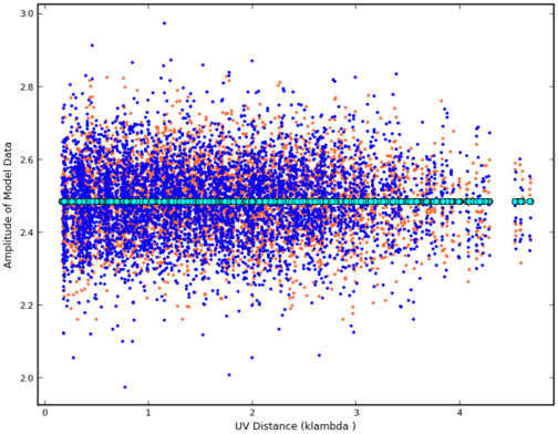\n",
"\n",
"Type Figure 1: ID Plot visualizing the corrected data (red and blue points) and the uv model fit (green circles). This particular plot was made using **plotxy**, which was deprecated in CASA 5.1 - use **plotms** instead.
\n",
"\n",
"\n",
"**Bibliography**\n",
"\n",
"1. Marti-Vidal, I., Vlemmings, W.H.T., Muller, S., & Casey, S. 2014, A&A, 563, A136 ([ADS](http://adsabs.harvard.edu/abs/2014A%26A...563A.136M))\n",
"1. Marti-Vidal et al. 2014, A&A 563, 136 ([arXiv:1401.4984](http://arxiv.org/abs/1401.4984))\\\n",
"\n",
"\n",
"\n",
"\n",
"\n"
]
}
]
}