\n",
"```\n",
"\n",
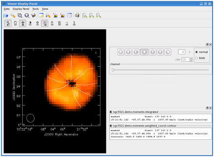
"Here we have contours spaced evenly from min to max, and this is what you get by default if you load a non-intensity image (like the moment-1 image).\n",
"\n",
"\n",
"**Overlay Contours on a Raster Map**\n",
"\n",
"Contours of either a second data set or the same data set can be used for comparison or to enhance visualization of the data. The Data Display Options Panel will have multiple tabs (switch between them at the top of the window) that allow you to adjust each overlay individually.\n",
"\n",
"\n",
"**NOTE**: Axis labeling is controlled by the first-registered image overlay that has labeling turned on (whether raster or contour), so make label adjustments within that tab.\n",
"
\n",
"\n",
"To add a Contour overlay, open the Load Data panel (Use the Data menu or click on the folder icon), select the data set and click on contour map.\n",
"\n",
"\n",
"\n",
"\n",
"**Creating a Position/Velocity Diagram**\n",
"\n",
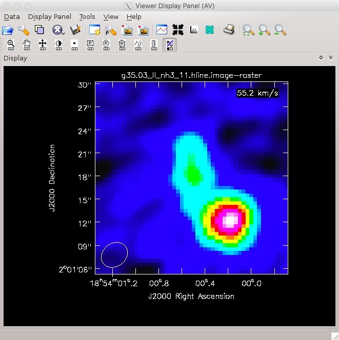
"With an image cube loaded, it is possible to create a position/velocity diagram using the P/V Button Tool. The first step in creating a P/V diagram is to select the tool with the mouse button to which you would like to bind the tool:\n",
"\n",
"\n",
"\n",
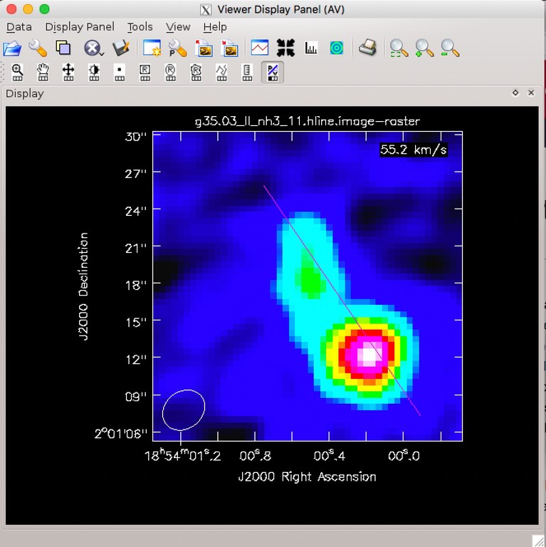
"Here we have bound the P/V button tool to the first mouse button. At this point, we can drag out a P/V line, by clicking and dragging on the image:\n",
"\n",
"\n",
"\n",
"\n",
"After creating the P/V line, it will appear with two circles on each end. These circles can be used to adjust the line by clicking within the circle and dragging:\n",
"\n",
"\n",
"\n",
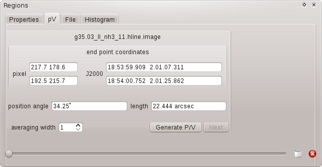
"After the P/V line is properly in place, the final P/V diagram can be created from the P/V Regions panel. It is just a matter of generating the P/V diagram with the Generate P/V button:\n",
"\n",
"\n",
"\n",
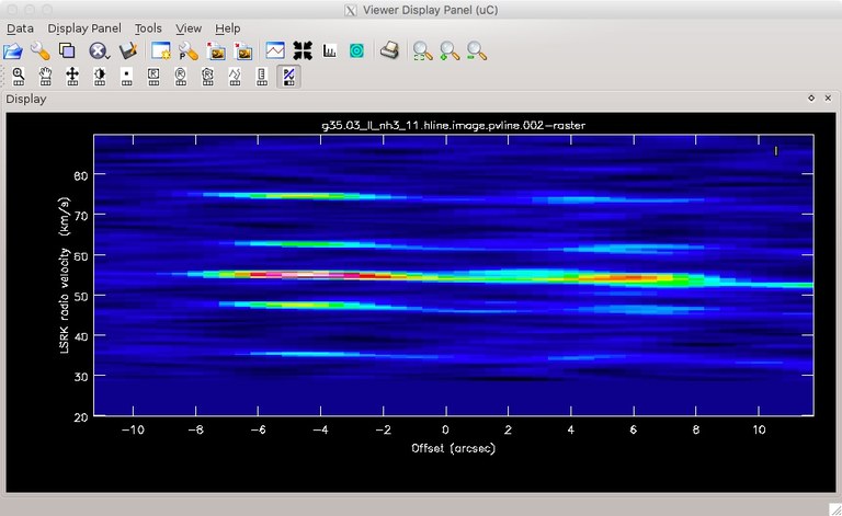
"The generation of the P/V diagram may take some time, but then the final diagram is displayed:\n",
"\n",
"\n",
"\n",
"\n",
"\n",
"***\n",
"\n",
"\n"
]
},
{
"cell_type": "markdown",
"metadata": {
"id": "gWxOO_fekunb"
},
"source": []
},
{
"cell_type": "markdown",
"metadata": {
"id": "2-UnZQkpkunb"
},
"source": [
"## Regions in the Viewer\n",
"\n",
"**Regions and the Region Manager**\n",
"\n",
"\n",
"\n",
"\n",
"CASA regions are following the CASA \\'crtf\\' standard as described in § [D](https://casa.nrao.edu/docs/cookbook/casa_cookbook015.html#chapter%3Aregionformat). CASA regions can be used in all applications, including **tclean** and [Image Analysis Tasks](image_analysis.ipynb).\n",
"\n",
"\n",
"**NOTE:** The CASA image analysis tasks will determine how a region is projected on a pixel image. The current CASA definition is that when the center of a pixel is inside the region, the full pixel is considered to be included in the region. If the center of the pixel is outside the region, the full pixel will be excluded. Note that the CASA viewer behavior is not entirely consistent and for rectangles it assumes that *any* fractional pixel coverage will include the entire pixel. For other supported shapes (ellipses and polygons), however, ithe viewer adheres to the 'center of pixel' definition, consistent with the image analysis tools and tasks.\n",
"\n",
"For purely single-pixel work regions may not necessarily be the best choice and alternate methods may be preferable to using regions, eg. **ia.topixel**, **ia.toworld**, **ia.pixelvalue**.\n",
"
\n",
"\n",
"\n",
"**ALERT:** Some region file specifications are not recognized by the viewer, the viewer only supports rectangles (box), ellipses, and polygons.\n",
"
\n",
"\n",
"\n",
"**NOTE**: A leading 'ann' (short for annotation) to a region definition indicates that it is for visual overlay purposes only.\n",
"
\n",
"\n",
"\n",
"**NOTE**: Whereas the region format is supported by all the data processing tasks, some aspects of the viewer implementation are still limited to rectangles, ellipses, and some markers. Full support for all region types is progressing with each CASA release.\n",
"
\n",
"\n",
"Once one or more regions are created, the Region Manager Panel becomes active. Like the Position Tracking and Animator Panels, this can be docked or detached from the main viewer display. It contains several tabs that can be used to adjust, analyze, and save or load regions.\n",
"\n",
"\n",
"**NOTE**: Moving the mouse into a region will bring it into focus for the Spectral Profile or Histogram tools.\n",
"
\n",
"\n",
"\n",
"**Region Creation, Selection, and Deletion**\n",
"\n",
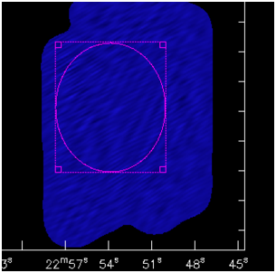
"Within the display area, you can draw regions or select positions using the mouse. Regions can be created with the buttons marked as \\'R\\' in the mouse tool bar, which can be found on the top-left (second row of buttons) in the [Viewer Display Panel](image_visualization.ipynb#viewer-basics). The viewer currently supports creation of rectangles, ellipses, polygons, and the point. As usual, a mouse button can be assigned to each button as indicated by the small black square in each button (marking the left, middle, or right mouse button).\n",
"\n",
"Regions can be selected by SHIFT+click, de-selected by pressing SHIFT+click again. The bottom of the Region Manager Panel features a slider to switch between regions in the image. Regions can be removed by hovering over and pressing ESC or by pressing the buttons to the right side of the slider where the first button (trash can icon) deletes all regions and the far right button (red circle with a white X) deletes the region that is currently displayed in the panel.\n",
"\n",
"\n",
"\n",
"\n",
"Once regions are selected, they will feature little, skeletal squares in the corners of their boundary boxes. Selected regions can be moved by dragging with the mouse button and manually resized by grabbing the corners as handles. If more than one region is selected, all selected regions move together.\n",
"\n",
"The Rectangle Region drawing tool currently enables the full functionality of the various Region Manager tabs (see below) as well as:\n",
"\n",
"- Region statistics reporting for images via double clicking (also shown in the Statistics tab of the Region Manager),\n",
"- Defining a region to be averaged for the spectral profile tool (accessed via the Tools:Spectral Profile drop down menu or \\\"Open the Spectrum Profiler\\\" icon),\n",
"- Flagging of MeasurementSets. Note that the Rectangle Region tool's mouse button must also be double-clicked to confirm an MS flagging edit.\n",
"- Selecting Clean regions interactively (§ [5.3.5](https://casa.nrao.edu/docs/cookbook/casa_cookbook006.html#section%3Aim.clean.interactive))\n",
"\n",
"The Polygon Region and Ellipse Region drawing have the same uses, except that polygon region flagging of a MeasurementSet is not supported.\n",
"\n",
"\n",
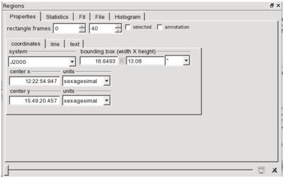
"**Region Positioning**\n",
"\n",
"\n",
"\n",
"\n",
"\n",
"With at least one region drawn, the Region Manager becomes active. Using the Properties tab, one can manually adjust the position, annotation, and display style of the region. The entries labeled \\\"frames\\\" set which planes of the image cube the region persists through (regions can have a depth associated with them and will only appear in the frames listed in this range). One can manually adjust the width and height and the center of the box in the chosen units. The \\'selected\\' check box is an alternative way to the SHIFT+click to select a region. The \\'annotation\\' checkbox will place the \\\"ann\\\" string in front of the region ASCII output -- annotation regions are not be used for processing in, e.g. data analysis tasks. In the line and text tabs, one can set the style with which the region is displayed, the associated text, and the position and style of that text.\n",
"\n",
"\n",
"**NOTE**: Updating the position of a region will update the spectral profile shown if the Spectral Profile tool is open and the histogram if the Histogram tool is open. The views are linked. Dragging a region or adjusting it manually with the Properties tab is a good way to explore an image.\n",
"
\n",
"\n",
"\n",
"**Region Statistics**\n",
"\n",
"\n",
"\n",
"\n",
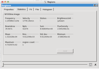
"One of the most useful features of defining a region is the ability to extract statistics characterizing the intensity distribution inside the region. You can see these in the Statistics tab of the of the Region Manager Panel. This displays statistics for the current region in the current plane of the current image. When more than a single region is drawn, you can select them one by one and the Region Panel will update the statistics to reflect the currently selected region. All values are updated on the fly when the region is dragged across the image.\n",
"\n",
"A similar functionality can be achieved by double clicking inside of a region. This will send statistics information for this region in all registered images to the terminal, looking something like this:\n",
"\n",
"```\n",
"(IRC10216.36GHzcont.image) image\n",
" Stokes Velocity Frame Doppler Frequency\n",
" I -2.99447e+11km/s LSRK RADIO 3.63499e+10\n",
" BrightnessUnit BeamArea Npts Sum Flux\n",
" Jy/beam 36.2521 27547 1.087686e-01 3.000336e-03\n",
" Mean Rms Std dev Minimum Maximum\n",
" 3.948473e-06 3.723835e-04 3.723693e-04 -1.045624e-03 9.968892e-03\n",
"```\n",
"\n",
"Listed parameters are Stokes, and the displayed channel Velocity with the associated Frame, Doppler and Frequency value. Sum, Mean, Rms, Std Deviation, Minimum, and Maximum value refer to those in the selected region and has the units as specified in BrightnessUnit. Npts is the number of pixels in the region, and BeamArea the beam size in pixels. FluxDensity is in Jy if the image is in Jy/beam. This is an easy way to copy and paste the statistical data to a program outside of CASA for further use.\n",
"\n",
"Taking the RMS of the signal-free portion of an image or cube is a good way to estimate the noise. Contrasting this number with the maximum of the image gives an estimate of the dynamic range of the image. The FluxDensity measurement gives a way to use the viewer to do very basic photometry.\n",
"\n",
"\n",
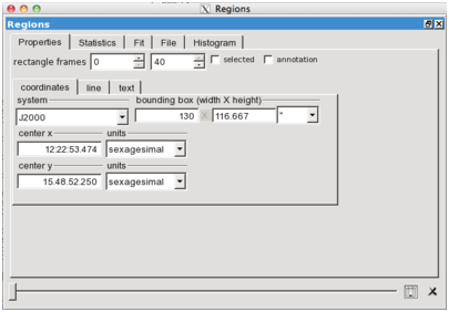
"**Saving and Loading Regions**\n",
"\n",
"\n",
"\n",
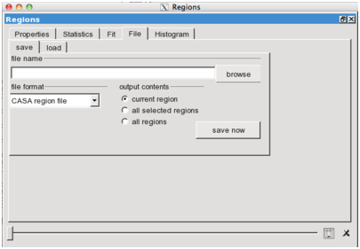
"The File tab in the Region Manager allows one to save or load selected regions, either individually or en masse. You can choose between CASA and DS9 region format. The default is a CASA region file (saved with a \\'.crtf\\' suffix, see § [D](https://casa.nrao.edu/docs/cookbook/casa_cookbook015.html#chapter%3Aregionformat)). The DS9 format does not offer the full flexibility and cannot capture Stokes and spectral axes. DS9 regions will only be usable as annotations in the viewer, they cannot be used for data processing in other CASA tasks. When saving regions, one can choose to save only the current region, all regions that were selected with SHIFT+click, or all regions that are visible on the screen.\n",
"\n",
"\n",
"**NOTE**: The load functionality for this tab will only become available once at least one region exists. To load a region when no regions exist, use the *Region Manager* window.\n",
"
\n",
"\n",
"\n",
"**The Region Fit**\n",
"\n",
"The Viewer can attempt to fit a two-dimensional Gaussian to the emission distribution inside the currently selected region. To attempt the fit, go to the Fit tab of the Region Manager and click the \\'gaussfit\\' button in the bottom left of the panel. You can choose whether or not to fit a sky level (e.g., to account for a finite background, either astronomical, sky, or instrumental). After fitting the distribution, the Fit panel shows the results of the fit, the center, major and minor axis, and position angle of the Gaussian fit in pixels (I) and in world coordinates (W, RA and Dec). The detailed results of the fit will also appear in the terminal window, including a flag showing whether the fit converged.\n",
"\n",
"\n",
"**The Region Histogram**\n",
"\n",
"\n",
"\n",
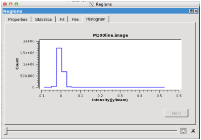
"> Histogram Tab: The histogram tab in the Region Manager. Right click to zoom. Hit SHIFT + Right Click to adjust the details of the histogram display.\n",
"\n",
"The viewer will automatically derive a histogram of the pixel values inside the selected region. This can be viewed using the Histogram tab of the of the Region Manager Panel. This is a pared down version of the full Histogram Tool. You can manipulate the details of the histogram plot by:\n",
"\n",
"1. Using the Right Click to zoom - either to the full range, a selected percentile, or a range that you have graphically selected by dragging the mouse.\n",
"2. Hitting SHIFT + Right Click to open the histogram options. This lets you toggle between a logarithmic and linear y-axis, choose between a line, outline, or filled histogram, and adjust the number of bins.\n",
"\n",
"The histogram will update as you change the plane of the cube or shift between regions.\n",
"\n",
"***\n",
"\n",
"\n",
"\n"
]
},
{
"cell_type": "markdown",
"metadata": {
"id": "lsy6bHjzkunc"
},
"source": [
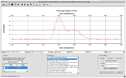
"## Spectral Profiler\n",
"\n",
"\n",
"\n",
"\n",
"**NOTE**: Make Sure That You Use the Radio Version! This section describes the 'Radio' version of the profiler. To be sure that you have the radio version of the tool selected (this may not be the default), click on the preferences icon (the 'gear' fourth from the left in the Spectral Profile tool) and make sure that the 'Optical' option is not checked. If you are using the Spectral Profile tool in the viewer for the very first time, you will also be prompted for a selection that will subsequently be kept for all future calls unless the preference is changed.\n",
"
\n",
"\n",
"The Spectral Profile Tool consists of the *Spectral Profile Toolbar*, a main display area, and two associated tabs: *Spectral-Line Fitting* and *Line Overlays*.\n",
"\n",
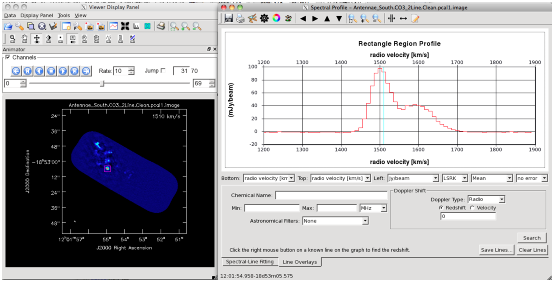
"Interaction With the Main Display Panel: For the Spectral Profile tool to work, a region or point must be specified in the main Viewer Display window. Use the mouse tools to specify a point, rectangle, ellipse, or polygon region. Alternatively, load a region file. The Spectral Profile tool will show a spectrum extracted from the region most recently highlight by the mouse in the main Viewer Display Panel. The method of extraction (i.e. mean, median, sum, or flux density) can be specified by the user using a drop down menu below the spectrum in the Spectral Profile window; the method of extraction is mean by default.\n",
"\n",
"The Spectral Profile tool can also feed back to the Main Display Panel. By holding CTRL and right clicking in the spectrum, you will cause the Main Display Panel to jump to display the frequency channel corresponding to the spectral (x) coordinate of the region highlighted in the Spectral Profile tool. Holding CTRL and dragging out a spectral range while holding the right mouse button will queue a movie scrolling through images across that spectral range. You can achieve the same effect with the two-ended-arrow icon towards the right of the toolbar in the Spectral Profile window.\n",
"\n",
"In both the *Spectral-Line Fitting* and *Line Overlays* tabs, it may be useful to select a range in frequency or velocity. You can do this with the parallel lines-and-arrow icon (see below) or by holding shift, left clicking, and dragging out the range of interest. A shaded gray region should appear indicating your selection.\n",
"\n",
"\n",
"**Spectral Profile Toolbar**\n",
"\n",
"\n",
"\n",
">Spectral Profile Toolbar: The toolbar for the Spectral Profile tool allows the user to save the spectrum, print or save the tool as an image, edit preferences (general, tool, legend), apply spectral smoothing, pan or zoom around the spectrum, select a range of interest, jump to a channel, or add a label.\n",
"\n",
"\n",
"The *Spectral Profile Toolbar* is the toolbar along the top of the Spectral Profile window. From left to right, the icons allow the user to:\n",
"\n",
"- (disk) export the current profile to a FITS or ASCII file\n",
"- (printer) print the main window to a hard copy\n",
"- (writing desk) save the panel as an image (PNG, JPG, PDF, etc.)\n",
"- (gear) set plot preferences\n",
"- (color wheel) set color preferences for the plot\n",
"- (signpost) set legend preferences\n",
"- (triangle) set the spectral smoothing method and kernel width\n",
"- (arrows) pan the spectrum in the indicated direction NOTE: The arrow keys also allow one to pan using the keyboard.\n",
"- (magnifying glass) zoom to the default zoom, in, and out NOTE: the +/- keys allow one to zoom with the keyboard\n",
"- (parallel lines+arrows) drag out a range of interest in the spectrum, for use with fitting or line overlays.\n",
"- (double-ended arrow) jump to a channel in the main viewer (single click) or define a range over which to play a movie in the viewer (with a drag).\n",
" \n",
"\n",
"**NOTE**: You can also jump to a channel with CTRL+Right Click and queue a movie by holding CTRL and dragging out a range while holding the right mouse button.\n",
"
\n",
"\n",
"- (notepad and pencil) Add or edit a label on the plot. Click this icon to enter a mode where you can drag out a box to create a new annotation box or drag the corners of an existing one to resize it. You can edit the contents, color, and font of an existing annotation by right clicking on it and selecting \\\"Edit Annotation\\\" in the main Spectral Profile window.\n",
"\n",
"\n",
"\n",
"*Spectral Profile Tool Preferences* shows the setting dialogs accessible from the toolbar. This Preferences dialog opened by the \\'gear\\' icon allows the user to:\n",
"\n",
"- Toggle automatic scaling the x- and y-ranges of the plot.\n",
"- Toggle the coordinate grid overlay in the background of the plot.\n",
"- Toggle whether registered images other than the current one appear as overlays on the plot.\n",
"- Toggle whether these profiles are plotted relative to the main profile (in development).\n",
"- Toggle the display of tooltips (in development).\n",
"- Toggle the plotting of a top axis.\n",
"- Toggle between a histogram and simple line style for the plot.\n",
"- Toggle between the radio and optical versions of the Spectral Profile tool Note: We discuss only the radio version here; this mainly impacts the Spectral Line Fitting and Collapse/Moments functionality..\n",
"- Toggle the overplotting of a line showing the channel currently being displayed in the main Display Panel.\n",
"\n",
"The Color Curve Preferences dialog opened by the \\'color wheel\\' icon allows the user to:\n",
"\n",
"- Select the color of the line marking the current channel shown in the main Display Panel.\n",
"- Select the color used to overlay molecular lines from Splatalogue.\n",
"- Select the color to plot the initial Gaussian estimate used in spectral line fitting.\n",
"- Select the color used for the zoom rectangle.\n",
"- Set a queue of colors used to plot the various data sets registered in the Display Panel.\n",
"- Set a queue of colors to plot the set of Gaussian fits.\n",
"- Set a queue of colors to plot the synthesized curve.\n",
"\n",
"Two sets of preset colors, \\\"Traditional\\\" or \\\"Alternative\\\", are available or the user can define their own custom color palette.\n",
"\n",
"The legend options opened by the \\'signpost\\' icon allow the user to toggle the plotting of a legend defining the curves shown in the main Spectral Profile window. Using a drop-down dialog, the legend can be placed in the top left corner of the plot, to the right of the plot, or below the plot. Toggling the color bar causes the color of the curve to be indicated either via a short bar or using the color of the text itself. Double click the names of the files or curves to edit the text shown for that curve by hand. A legend is only available if more than a single spectrum has been loaded.\n",
"\n",
"The spectral smoothing option (triangle icon in the Spectral Profile toolbar) has two methods, \\\"Boxcar\\\" and \\\"Hanning\\\" with the selection of odd numbers for the smoothing kernel width in channels.\n",
"\n",
"\n",
"**Main Spectral Profile Window**\n",
"\n",
"\n",
"\n",
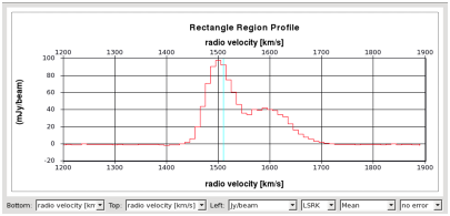
"The main window shows the spectrum extracted from the active region of the image in the main Display Panel. The spectra from the same region in any other registered images are also plotted if overlays are enabled. Menus along the bottom of the image allow the user to select how the spectrum is displayed. From left to right:\n",
"\n",
"- The units for the bottom spectral axis.\n",
"- The units for the top spectral axis.\n",
"\n",
"\n",
"**NOTE**: Dual axes are enabled only if a single image is registered and the top axis option is enabled. In general, dual axes are not well-defined for mixed data sets. The exception is that open data cubes with matched frequency/spectral axes will allow dual axes.\n",
"
\n",
"\n",
"- The units for the left intensity or flux axis\n",
"\n",
"\n",
"**NOTE**: The \"Fraction of Peak\" option allows for easy comparison of data with disparate intensity scales.\n",
"
\n",
"\n",
"- The velocity reference frame used if a velocity axis is chosen for the top or bottom axis.\n",
"- The method used to extract spectrum from the region --- a mean over all pixels in the region, a median, sum, or a sum converting units to get a flux density over the region (Jy).\n",
"- Toggle the calculation and overplotting of error bars calculated from scatter in the data (rmse refers to root mean square error).\n",
"\n",
"In addition to these drop-down menus, the main Spectral Profile window allows the user to do the following using keyboard and mouse inputs:\n",
"\n",
"- jump the main Display Panel window to a specified channel (CTRL+Right click): hold CTRL and right click in the spectrum. A marker will appear and the main Viewer Display Panel will jump to display that channel.\n",
"- animate the main Display Panel in a movie across a frequency range (CTRL+Right click+drag): hold CTRL, Right click, and drag. The main Viewer Display panel will respond by showing a movie scrolling across the selected spectral channels.\n",
"- zoom the Spectral Profile (+/-, mouse drag): Use the +/- keys to zoom in the same way as the toolbar buttons. Alternatively, press and drag the left mouse button. A yellow box is drawn onto the panel. After releasing the mouse button, the plot will zoom to the selected range.\n",
"- pan the Spectral Profile (arrows): Use the arrow keys to pan the plot.\n",
"- select a spectral range for analysis: hold shift, left click, and drag. A gray area will be swept out in the display. This method can be used to select a range for spectral line fitting or collapsing a data cube (in the Collapse/Moments window).\n",
"\n",
"**NOTE**: If the mouse input to the Spectral Profile browser becomes confused hit the ESC key several times and it will reset.\n",
"\n",
"\n",
"**Spectral-Line Fitting**\n",
"\n",
"\n",
"\n",
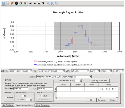
">Spectral Line Fitting Tab: Using the Spectral Line Fitting Tab (found at the bottom left of the Spectral Profile Tool), the user can fit a combination of a polynomial and multiple Gaussian components. The range to be fit can be specified (gray region) manually or with a shift+click+drag. Initial estimates for each component may be entered by hand or specified via an initial estimates GUI. The results are output to a dialog and text file with the fit overplotted (here in blue) on the spectrum (with the possibility to save it to disk).\n",
"\n",
"\n",
"\n",
"\n",
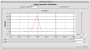
">Specifying Initial Gaussian Estimates Graphically and Fitting Output: The top panel shows the graphical specification of initial estimates for Gaussian fitting. Slider bars specify the center, FWHM, and peak intensity for the initial estimate. The bottom panel shows the verbose output of the fitting.\n",
"\n",
"\n",
"The Spectral-Line Fitting tab allows the user to interactively fit a combination of Gaussian and polynomial profiles to the data shown in the Spectral Line Profile tool. The tool includes a number of options:\n",
"\n",
"- A drag-down menu labeled \\\"Curve\\\" at the top of the panel allows the user to pick which data set to fit.\n",
"- The spectral range to fit can be specified by either holding shift+left click+dragging out a region in the main spectral profile window or by typing it manually into the boxes labeled Min and Max near the top left of the fitting panel.\n",
"- Optionally multiple fits can be carried out once, fitting each spectrum in the region in turn. To enable this, check the \\'MultiFit\\' box.\n",
"- Optionally a polynomial of the specified order may be fit. To do so, check the \\'Polynomial\\' fit check box and then specify the desired order.\n",
"- The results may be saved to a text file. This text file should be specified before the fit is carried out. Click \\'Save\\' and then use the dialog to specify the file name. Note that the fit curve itself becomes a normal spectral profile data set and can be saved to disk using the toolbar (\\'disk\\' icon) after the fit.\n",
"- One or more Gaussians can be fit, although results are presently most stable for one Gaussian. Specify the number of Gaussians in the box marked \\\"Gaussian Count\\\" and then enter initial estimates for the peak, center, and FWHM in the table below. Any of these values can be fixed for any of the Gaussians being fit. Initial estimates can also be manually specified by clicking \\\"Estimates\\\". This brings up an additional GUI window, where sliders can be used to specify initial estimates for each Gaussian to be fit.\n",
"- For plotting purposes, one may wish to oversample the fit (i.e., plot a smooth Gaussian), you can do so by increasing the Fit Samples/Channel to a high number to finely sample the fit when plotting.\n",
"\n",
"**NOTE**: Currently the tool works well for specifying a single Gaussian. Fitting multiple Gaussian components can become unstable.\n",
"\n",
"\n",
"**Line Overlays**\n",
"\n",
"\n",
"\n",
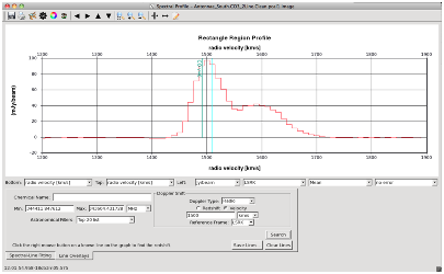
">Line Overlays Tab: The Line Overlay tab (found at the bottom left of the Spectral Profile Tool) allows users to query the CASA copy of the Splatalogue spectral line database. Enter the redshift of your source (far right of the panel), select an Astronomical Filter from the drop down menu, and use shift+click+drag to select a frequency range (or enter the range manually in the boxes marked Min and Max). The \\\"Search\\\" button will bring up a separate \\\"Search Results\\\" window, which can in turn be used to graph the candidate lines in the main Spectral Profile window (here CO v=0).\n",
"\n",
"\n",
"Each version of CASA includes a local version of the [Splatalogue](http://www.splatalogue.net) spectral line database and this can be used to identify and overplot spectral transitions. This feature, shown in *Line Overlay Tab*, allows the user to search Splatalogue over the range of interest.\n",
"\n",
"To overlay spectral lines:\n",
"\n",
"1. Select the Line Overlays tab in the Spectral Profiles tab.\n",
"2. If you know it, enter the redshift or velocity of your source in the \\\"Doppler Shift\\\" panel. Otherwise, the lines will be overlaid assuming a redshift of 0.\n",
"3. Specify a minimum and maximum frequency range to search, either by typing a range or by holding shift and left click and dragging out a range in the spectrum (you will see a gray box appear). If you don't specify a range, the tool will search over the frequency range of spectrum.\n",
"4. Optionally, you may select an astronomical filter from the list (e.g., commonly used extragalactic lines or lines often found in hot cores, see [Splatalogue](http://www.splatalogue.net) for more information). This is usually a good idea because it pares the potentially very large list of candidate lines to a smaller set of reasonable candidates.\n",
"5. Click \\'Search\\' and the Spectral Profile will search Splatalogue for a list of Spectral lines that fit the selected Astronomical Filter in the selected frequency range for the selected redshift. A \\\"Molecular Line Search Results\\\" dialog box will pop up showing the list of candidate lines.\n",
"6. Highlight one or more of these transitions and click \\'Graph Selected Lines\\'. A set of vertical markers will appear in the main Spectral Profile window at the appropriate (redshifted) frequencies for the line.\n",
"\n",
"NOTE: You will want to click \\'Clear Lines\\' between searches, especially if you update the redshift.\n",
"\n",
"\n",
"**The Collapse/Moments Tool**\n",
"\n",
"\n",
"\n",
"\n",
"\n",
"The CASA Viewer (**imview**) can collapse a data cube into an image, for instance allowing to look at the emission integrated along the z axis or the mean velocity of emission along the line of sight. You can access this functionality via the Collapse/Moments tool (accessed via the Tools drop down menu in the Main Display planel or via the four inward pointing arrows icon in the Main Toolbar) which is shown in *Collapse/Moments Tool*.\n",
"\n",
"The tool uses the same format as the Spectral Profile tool and will show the integrated spectrum of whatever region or point is currently selected in the Main Display Panel. To create a moment map:\n",
"\n",
"1. Select a range over which to integrate either manually using the left part of the window, by adding an interval and typing in the values into the boxes marked Min and Max or by holding SHIFT + Left Click and dragging out the range of interest.\n",
"2. Pick the set of algorithms (listed in the box labeled \\\"Moment(s)\\\") that you will use to collapse the image along the z-axis. Clicking an option toggles that moment method, and the collapse will create a new image for each selected moment. For details on the individual collapse method, see the [immoments](../api/casatasks.rst) task for more details on each moment.\n",
"3. The moment may optionally include or exclude pixels within a certain range (for example, you might include only values with signal-to-noise of three or greater when calculating the velocity dispersion). You can enter the values to include or exclude manually in the Thresholding window on the right or you can open a histogram tool to specify this range graphically by clicking Specify Graphically (before this can work, you must click \\'Include\\' or \\'Exclude\\').\n",
"4. The results of the collapse can be saved to a file, which consists of a string specifying the specific moment tacked onto a root file name that you can specify using Select Root Output File.\n",
"5. When you are satisfied with your chosen options, press \\'Collapse\\'.\n",
"\n",
"**NOTE**: Even if you don't save the results of the collapse to a file, you can still save the map later using the Save as\\... entry in the Data pull down menu from the Main Viewer Display Panel.\n",
"\n",
"\n",
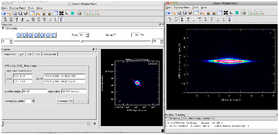
"**Interactive Position-Velocity Diagram Creation**\n",
"\n",
"\n",
"\n",
"\n",
"The route to create position-velocity cuts in the viewer is illustrated in *Position/Velocity Tool*:\n",
"\n",
"1. Select the \\'P/V cut\\' tool from the Mouse Toolbar and use it to draw a line across a data cube along the axis you want to visualize.\n",
"2. Open the Region Manager Panel and go to the pV tab. Highlight the cut you just drew. You should see the end point coordinates listed, along with information on the length and position angle of the cut. You can set the averaging width (in pixels) in a window at the bottom of the tab.\n",
"3. When you are satisfied, hit \\'Generate P/V\\'. This will create a new Main Viewer Display Panel showing the position velocity cut. The axes should be Offset and velocity.\n",
"\n",
"The new image can be saved to disk with the Data\\\\:Save as\\... option.\n",
"\n",
"\n",
"***\n",
"\n",
"\n",
"\n"
]
},
{
"cell_type": "markdown",
"metadata": {
"id": "2nMaIr4ykunc"
},
"source": [
"## Image Analysis in the Viewer (imview)\n",
"\n",
"Analysis Tools that are available in the Viewer (task **imview**).\n",
"\n",
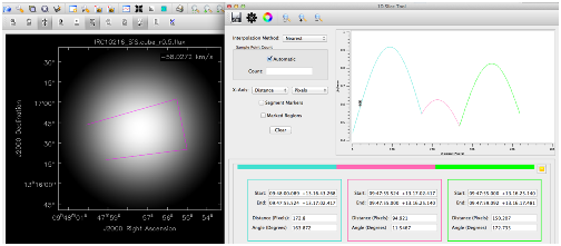
"**The Brightness Profile Tool**\n",
"\n",
"The viewer allows the user to draw multiple line segments using the \\\"Polyline drawing\\\" button, and this feature can be used to display one-dimensional brightness profiles of images, such as shown in the *Spatial Profile Tool*. After double-clicking the last line segment, the \\'Regions\\' dock will then display a preview of the slice in the Spatial Profile tab and the full \\\"Spatial Profile Tool\\\" can be launched from there by clicking the \\\"Spatial Profile Tool\\\" button. This \\\"Spatial Profile Tool\\\" panel allows one to select the interpolation method to connect the pixels, and a number count for the sampled pixels in between markers. \\'Automatic\\' will show all pixels. The x-axis of the display can be either the distance along the slice or the X and Y coordinate projections (e.g. along RA and DEC). All segments are also listed at the bottom with their start and end coordinates, the distance and the position angles of each slice segment. The color tool can be used to give each segment a separate color.\n",
"\n",
"\n",
"\n",
"\n",
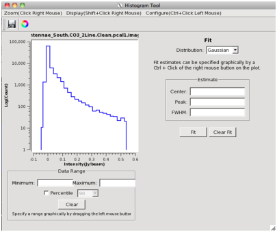
"**The Histogram Tool**\n",
"\n",
"\n",
"\n",
"CASA can calculate and visualize a histogram of pixel values inside a region of interest. To examine this histogram, select Histogram from the Tools drop-down menu or the \\'Histogram\\' icon in the Main Toolbar (looks like a comb). This opens the full Histogram Tool; more limited versions are accessible from the Region Manager Panel, the graphical color table manipulation tool, and the Collapse/Moments tool.\n",
"\n",
"The resulting Histogram Tool should look something like *Histogram Tool*. The menus along the top (or the corresponding mouse clicks) allow one to:\n",
"\n",
"- Zoom to the full range, a selected percentile, or a graphical range.\n",
"- Change the display of the histogram to show a log axis, display as either a line plot, an outline, or a filled histogram. Change the number of bins in the histogram, or clear the plot (to start over).\n",
"- Configure what data are fed into the histogram. You can use this menu to tell the histogram to track the channel currently selected in the main Viewer Display Panel (click the \\\"Track Channel\\\" box) or to integrate across some range of channels (defaulting to the whole image). You can also switch the 2-D footprint used between the whole Image, the Selected Region, and All Regions.\n",
"- Save (via the disk icon) an image of the histogram to a graphical file on disk.\n",
"\n",
"The Histogram Tool also allows you to fit the distribution using either a Gaussian or a Poisson distribution, for example to estimate the noise in the image (a Gaussian will be a good choice to describe the noise in most radio data cubes). You can specify initial estimates or let the program generate initial guesses. The fit is then overplotted on the histogram (colors can be adjusted by clicking the color wheel icon in the toolbar) and details of the fit are printed to the text window below the fit button.\n",
"\n",
"\n",
"**The Two-Dimensional Fitting Tool**\n",
"\n",
"\n",
"\n",
"\n",
"CASA can fit two-dimensional Gaussians to an intensity distribution, and the Two-Dimensional Fitting Tool in the Viewer exposes this functionality interactively. This tool, accessed by the \\'blue circles\\' icon in the Main Toolbar or the Tools:Fit menu item, has an interface like that shown in *Two-Dimensional Fitting Tool*. The interface exposes several options:\n",
"\n",
"\n",
"**NOTE**: The two dimensional fitter only operates on a single channel at a time.\n",
"
\n",
"\n",
"1. You can select whether to fit only the selected region or the whole image plane and specify which channel of the cube you want to operate on.\n",
"2. Initial Estimates: The box in the top left corner allows the user to specify initial estimates by feeding in a file. The easiest way to make an appropriate file is to edit an existing one. Even easier, you can use the Find Sources button to automatically generate a temporary file of initial estimates.\n",
"3. Pixel Range: You can choose to only include a certain range of pixel intensity values in the fit. For example, you might choose to only fit Gaussians to pixels a few times above the measured noise level. You can use the Specify Graphically button to bring up an interactive histogram of the region (a reduced functionality version of the full Histogram Tool).\n",
"4. Output: You can choose to save the output of the fit as a file to the specified directory and to subtract the fit from the image and to subtract the fit from the original, creating a Residual Image that gets stored as a CASA image and automatically loaded into the viewer. This gives a way to tell how well your fit describes the total emission.\n",
"5. Visualization: You can toggle whether the fit is displayed on the viewer or not and change the color of the marker.\n",
"\n",
"Click Fit to start the fit. If the fit does not converge, try improving your initial estimates and fitting again.\n",
"\n",
"\n",
"***\n",
"\n",
"\n",
"\n",
"\n",
"\n"
]
},
{
"cell_type": "markdown",
"metadata": {
"id": "L-JRi8Vxkunc"
},
"source": [
"## Printing from the Viewer\n",
"\n",
"You can select Data\\\\:Print from the drop down menu or click the printer icon in the Main Toolbar to bring up the Viewer Print Manager. From this panel, you can \\\"Print\\\" the contents of Display Panel to a hardcopy or \\\"Save\\\" them as an image in a format selected from the drop-down menu at the bottom left of the window.\n",
"\n",
"\n",
"**NOTE**: The save feature will overwrite the file in question without prompting.\n",
"
\n",
"\n",
"The Viewer Print Manager allows you to adjust the DPI, orientation, and page format (Output Media) for Postscript or PDF files and to scale the image to a desired pixel size for other images.\n",
"\n",
"To achieve the best output it is usually advisable to adjust the settings in the Viewer Print Manager (printer icon in the Main Toolbar), Data Display Options (Data\\\\:Adjust Data Display), and Viewer Canvas Manager (wrench+\\\"P\\\" icon in the Main Toolbar). For PDF and Postscript output, turning the DPI up all the way yields the best-looking results. For other images, a white background often makes for better looking images than the default black. It is often necessary to increase the Line Width in the Axis Label Properties (in the Data Display Options panel) to ensure that the labels will be visible when printed. Increasing from the default of 1.4 to a value around 2 often works well.\n",
"\n",
"The following figure shows an example of printing to a file while adjusting the Data Display Options and Viewer Canvas Manager to improve the appearance of the plot.\n",
"\n",
"\n",
"\n",
"\n",
"***\n",
"\n",
"\n",
"\n"
]
},
{
"cell_type": "markdown",
"metadata": {
"id": "Bn5yvX1Okund"
},
"source": [
"## Scripting using imview\n",
"\n",
"\n",
"The **imview** task offers scriptable access to many **viewer** options. This enables the production of customized plots without invoking the GUI and allows one to open the **viewer** to a carefully selected state.\n",
"\n",
"**imview** has the following inputs:\n",
"\n",
"```\n",
"#imview :: View an image\n",
"raster = {} #(Optional) Raster filename (string)\n",
" #or complete raster config\n",
" #dictionary. The allowed dictionary\n",
" #keys are file (string), scaling\n",
" #(numeric), range (2 element numeric\n",
" #vector), colormap (string), and\n",
" #colorwedge (bool).\n",
"contour = {} #(Optional) Contour filename (string)\n",
" #or complete contour config\n",
" #dictionary. The allowed dictionary\n",
" #keys are file (string), levels\n",
" #(numeric vector), unit (float), and\n",
" #base (float).\n",
"zoom = 1 #(Optional) zoom can specify\n",
" #intermental zoom (integer), zoom\n",
" #region read from a file (string) or\n",
" #dictionary specifying the zoom\n",
" #region. The dictionary can have two\n",
" #forms. It can be either a simple\n",
" #region specified with blc (2 element\n",
" #vector) and trc (2 element vector)\n",
" #[along with an optional coord key\n",
" #(\"pixel\" or \"world\"; pixel is the\n",
" #default) or a complete region\n",
" #rectangle e.g. loaded with\n",
" #\"rg.fromfiletorecord( )\". The\n",
" #dictionary can also contain a\n",
" #channel (integer) field which\n",
" #indicates which channel should be\n",
" #displayed.\n",
"axes = -1 #(Optional) this can either be a\n",
" #three element vector (string) where\n",
" #each element describes what should\n",
" #be found on each of the x, y, and z\n",
" #axes or a dictionary containing\n",
" #fields \"x\", \"y\" and \"z\" (string).\n",
"out = {} #(Optional) Output filename or\n",
" #complete output config dictionary.\n",
" #If a string is passed, the file\n",
" #extension is used to determine the\n",
" #output type (jpg, pdf, eps, ps, png,\n",
" #xbm, xpm, or ppm). If a dictionary\n",
" #is passed, it can contain the\n",
" #fields, file (string), scale\n",
" #(float), dpi (int), or orient\n",
" #(landscape or portrait). The scale\n",
" #field is used for the bitmap formats\n",
" #(i.e. not ps or pdf) and the dpi\n",
" #parameter is used for scalable\n",
" #formats (pdf or ps).\n",
"```\n",
"\n",
"The *raster* and *contour* parameters specify which images to load and how these images should be displayed. These parameters take python dictionaries as inputs. The fields in these dictionaries specify how the image will be displayed.\n",
"\n",
"An example call to **imview** looks like this:\n",
"\n",
"```\n",
"imview(raster={'file': 'ngc5921.clean.image','range': [-0.01,0.03],'colormap': 'Hot Metal 2','scaling': -1},\n",
" contour={'file': 'ngc5921.clean.image'},\n",
" axes={'x':'Declination'},\n",
" zoom={'channel': 7, 'blc': [75,75], 'trc': [175,175],'coord': 'pixel'},\n",
" out='myout.png')\n",
"```\n",
"\n",
"The argument to *raster* is enclosed in the curly braces { }. Within these braces are a number of \\\"key\\\":\\\"value\\\" pairs. Each sets an option in the **viewer**, with the GUI parameter to set defined by the \\\"key\\\" and the value to set it to defined by \\\"value.\\\" In the example above, file='ngc5921.clean.image' sets the file name of the raster image, range= \\[-0.01,0.03\\] sets the range of pixel values used for the scaling.\n",
"\n",
"*contour* works similarly to *raster* but can accept multiple dictionaries in order to produce multiple contour overlays on a single image. To specify multiple contour overlays, simply pass multiple dictionaries (comma delimited) in to the *contour* argument:\n",
"\n",
"```\n",
"contour={'file': 'file1.image', 'levels': [1,2,3] }, {'file': 'file2.image', 'levels': [0.006, 0.008, 0.010] }\n",
"```\n",
"\n",
"*zoom* specifies the part of the image to be shown. The example above specifies a channel as well as the top right corner \\\"trc\\\" and the bottom left corner \\\"blc\\\" of the region of interest.\n",
"\n",
"*axes* defines what axes are shown. By default, the viewer will show 'x':'Right Ascension', 'y':'Declination' but one may also view position-frequency images.\n",
"\n",
"*out* defines the filename of the output, with the extension setting the file type.\n",
"\n",
"Currently, the following parameters are supported:\n",
"\n",
"```\n",
"raster -- (string) image file to open\n",
" (dict) file (string) => image file to open\n",
" scaling (float) => scaling power cycles\n",
" range (float*2) => data range\n",
" colormap (string) => name of colormap\n",
" colorwedge (bool) => show color wedge?\n",
"contour -- (string) file to load as a contour\n",
" (dict) file (string) => file to load\n",
" levels (float*N) => relative levels\n",
" base (numeric) => zero in relative levels\n",
" unit (numeric) => one in the relative levels\n",
"zoom -- (int) integral zoom level\n",
" (string) region file to load as the zoom region\n",
" (dict) blc (numeric*2) => bottom left corner\n",
" trc (numeric*2) => top right corner\n",
" coord (string) => pixel or world\n",
" channel (int) => channel to display\n",
" (dict) => record loaded\n",
" e.g., rg.fromfiletorecord( )\n",
"axes -- (string*3) dimension to display on the x, y, and z axes\n",
" (dict) x => dimension for x-axes\n",
" y => dimension for y-axes\n",
" z => dimension for z-axes\n",
"out -- (string) file with a supported extension\n",
" [jpg, pdf, eps, ps, png, xbm, xpm, ppm]\n",
" (dict) file (string) => filename\n",
" format (string) => valid ext (filename ext overrides)\n",
" scale (numeric) => scale for non-eps, non-ps output\n",
" dpi (numeric) => dpi for eps or ps output\n",
" orient (string) => portrait or landscape\n",
"```\n",
"\n",
"Examples are also found in `help imview`.\n",
"\n",
"\n",
"**Scripting using the viewer tool**\n",
"\n",
"The **viewer** tool may also be used to generate simple figures that can be directly saved to an output image file format (png, jpg, etc). Below is an example.\n",
"\n",
"```\n",
"def dispimage(imname=''):\n",
" qq = viewertool()\n",
" qq.load(imname)\n",
" qq.datarange(range=[-0.01,1.1])\n",
" qq.colormap(map='Rainbow 3')\n",
" qq.colorwedge(show=True)\n",
" qq.zoom(blc=[100,150], trc=[600,640])\n",
" qq.output(device='fig_trial.png',format='png')\n",
" qq.close()\n",
"```\n",
"\n",
"Note that only basic controls are available via the **viewertool** interface. For additional customization via a script, please see the following section describing \\\"Using Viewer state files within a script\\\".\n",
"\n",
"\n",
"**Using Viewer state files within a script**\n",
"\n",
"In order to access the full flexibility of the GUI interface in customizing the **viewer** settings and display options, a hand-crafted **viewer** state can be saved, edited, and subsequently restored/rendered via a script that then allows the saving of the figure to a file on disk.\n",
"\n",
"For example:\n",
"\n",
"Step 1 : Customize the **viewer** by hand. For example, choose to open an image, customize the display data ranges, choose a colormap, change axis label properties, change the units of the movie axis label, edit the panel background color, adjust margins and and resize the panel window.\n",
"\n",
"Step 2 : Click on the \\\"save viewer state\\\" button on the top control panel of the **viewer**. This will save a .rstr file, which is an xml file containing a complete description of the current state of the **viewer**. \n",
"\n",
"Step 3 : Edit the text xml file as required. The simplest operation is to search and replace the name of the CASA image being opened. More complex editing can be done via stand-alone editing scripts perhaps using standard python xml parser/editing packages.\n",
"\n",
"Step 4 : Restore the state of the **viewer** from the edited xml .rstr file, using the **viewertool** as follows to subsequently save a .png figure to disk.\n",
"\n",
"```\n",
"CASA <1>: vx = viewertool()\n",
"CASA <2>: x = vx.panel('mystate.rstr')\n",
"CASA <3>: vx.output('myfig.png',panel=x)\n",
"```\n",
"\n",
"(There are two interactive ways to restore the **viewer** state as well. The first is by starting up the **viewer** with no image chosen, and then clicking on the \\\"restore viewer state\\\" button and choosing this .rstr file to open. Alternately, the **casaviewer** can itself be opened by supplying this .rstr file as the \\'image\\' to open.)\n"
]
}
]
}