{
"nbformat": 4,
"nbformat_minor": 0,
"metadata": {
"colab": {
"name": "image_analysis.ipynb",
"provenance": [],
"toc_visible": true
}
},
"cells": [
{
"cell_type": "markdown",
"metadata": {
"id": "Qqs_CS-mkunf"
},
"source": [
"# Image Analysis\n",
"\n",
"\n",
"The task **viewer** is deprecated in lieu of **imview** and **msview**, which contain the same functionality. Please invoke the **imview** (**msview**) task for running the CASA Viewer to visualize images or image cubes (visibility data).\n",
"
\n"
]
},
{
"cell_type": "markdown",
"metadata": {
"id": "zZPoDSe7kunf"
},
"source": [
"## CASA Images\n",
"\n",
"CASA images are stored as tables and can be accessed with CASA tasks and tools. Image metadata can be listed and edited with the **imhead** task. Further processing includes the computation of statistics including spectral indices and polarization properties, transformation onto different spatial coordinates, spatial resolutions, and spectral frames, and many other processes (see the following section on [Dealing with Images](image_analysis.ipynb#dealing-with-images) for a description of tasks that operate on CASA images).\n",
"\n",
"\n",
"**Image Headers**\n",
"\n",
"Image Headers contain metadata on the observation -- e.g. the observing date, pointing position, object observed, etc., and the resulting image -- e.g. the restoring beam size, image intensity units, spatial coordinate system, spectral parameters, stokes parameters, etc. Header metadata tells the user what is in the image, and is used by **imview** and other tasks to set the data array on the correct spatial and spectral coordinates, assign the intensity values correctly, and otherwise properly handle the data cube.\n",
"\n",
"Image Headers can be accessed and edited via the **imhead** task and the **msmd** tool. Header data can also be inspected with the **casabrowser**. See the page on [Image Headers](image_analysis.ipynb#Image-Headers) for further details.\n",
"\n",
"\n",
"**Image Axes / Velocity Systems**\n",
"\n",
"CASA images typically have the following axis order (python indices are zero-based): Axis 0 = RA, 1 = DEC, 2 = Stokes, 3 = Frequency. The spatial axes can alternately contain GLON/GLAT or other coordinate systems. The spectral axis of images created in CASA is always in frequency units. In addition, one or more velocity systems can be *added* to relabel the spectral axis. When images are imported into CASA from FITS files rather than generated within CASA itself, the above conventions may not apply. See the page on [Image Import and Export](image_analysis.ipynb#Image-Import/Export) for further details on importing and exporting FITS files.\n",
"\n",
"The spatial and spectral axes in CASA images can be modified using CASA tasks and tools described in the [Reformat Images](image_analysis.ipynb#Reformat-Images) page.\n",
"\n",
"\n",
"**Image Masks**\n",
"\n",
"Internal Image Masks are stored as Boolean True/False cubes within the images themselves. There can be multiple masks stored in each data cube and one of them is defined to be the \\'default\\' mask. The default mask is the one visible when the image is displayed, e.g. in the CASA Viewer, and that is applied for operations on images. All masks have labels, such as mask0 etc. and they can be selected by specifying the image name followed by the mask name, separated by a colon. For example, \\'mask1\\' in \\'image.im\\' is used when specifying the image as \\'image.im:mask1\\'. Available masks can be listed with the task **makemask** which can also assign any mask as the default. The same task can also be used to export masks into separate CASA zero/non-zero cubes and to import such cubes as Boolean masks inside images. In addition, **makemask** enables the creation of masks from [image regions](image_analysis.ipynb#region-files). More information on masks is provided on the [Image Masks](image_analysis.ipynb#image-masks) and [LEL Masks](image_analysis.ipynb#Lattice-Expression-Language) sections.\n",
"\n",
"\n",
"**CASA Regions**\n",
"\n",
"CASA Regions can be specified through simple lists in LEL (e.g. ```region = 'box[[108pix, 108pix,], [148pix, 148pix]]')``` or through CASA Region Text Format (CRTF) files, which are text files that contain one or more regions with specific shapes (e.g. ellipses and rectangles), sizes, and other properties. These files can be used to specify the region of an image in which to operate, and they can easily be modified by the user or converted to CASA image masks (Boolean data cubes) using the **makemask** task. More information on CRTF files is available on the [Region Files](image_analysis.ipynb#region-files) section. \n",
"\n",
"***\n",
"\n",
"\n"
]
},
{
"cell_type": "markdown",
"metadata": {
"id": "SVAo3JI0kung"
},
"source": [
"## Dealing with Images\n",
"\n",
"Image cubes in CASA can be manipulated and analyzed in various ways mainly using tasks with an \\'im\\' prefix and with the **image** CASA tool. Frequently, the tasks and tools handle CASA, FITS, and MIRIAD images, but we recommend using images in the CASA format.\n",
"\n",
"In the following pages, useful image analysis tasks are introduced that span import/export tasks, image information, reformatting, mathematical operations, and spatial and spectral fitting. Available image analysis tasks include:\n",
"\n",
"- **imhead** --- summarize and manipulate the \"header\" information in a CASA image\n",
"- **imsubimage** --- Create a (sub)image from a region of the image\n",
"- **imcontsub** --- perform continuum subtraction on a spectral-line image cube\n",
"- **imfit** --- image plane Gaussian component fitting\n",
"- **immath** --- perform mathematical operations on or between images\n",
"- **immoments** --- compute the moments of an image cube\n",
"- **impv** --- generate a position-velocity diagram along a slit\n",
"- **imstat** --- calculate statistics on an image or part of an image\n",
"- **imval** --- extract the data and mask values from a pixel or region of an image\n",
"- **imtrans** --- reorder the axes of an image or cube\n",
"- **imcollapse** --- collapse image along one or more axes by aggregating pixel values along that axis\n",
"- **imregrid** --- regrid an image onto the coordinate system of another image\n",
"- **imreframe** --- change the frame in which the image reports its spectral values\n",
"- **imrebin** --- rebin an image\n",
"- **specsmooth** --- 1-dimensional smooth images in the spectral and angular directions\n",
"- **imsmooth** --- 2-dimensional smooth images in the spectral and angular directions\n",
"- **specfit** --- fit 1-dimensional Gaussians, polynomial, and/or Lorentzians models to an image or image region\n",
"- **specflux** --- Report details of an image spectrum.\n",
"- **plotprofilemap** --- Plot spectra at their position\n",
"- **rmfit** --- Calculation of rotation measures\n",
"- **spxfit** --- Calculation of Spectral Indices and higher order polynomials\n",
"- **makemask** --- image mask handling\n",
"- **slsearch** --- query a subset of the Splatalogue spectral line catalog\n",
"- **splattotable** --- convert a file exported from Splatalogue to a CASA table\n",
"- **importfits** --- import a FITS image into a CASA image format table\n",
"- **exportfits** --- write out an image in FITS format\n",
"\n",
"There are other tasks which are useful during image analysis. These include:\n",
"\n",
"- **imview** --- there are useful region statistics and image cube slice and profile capabilities in the viewer\n",
"\n",
"***\n",
"\n",
"\n",
"\n"
]
},
{
"cell_type": "markdown",
"metadata": {
"id": "ODANbAkJkung"
},
"source": [
"## Common Task Parameters\n",
"\n",
"Certain parameters are present in many image analysis tasks. These include:\n",
"\n",
"*imagename*\n",
"\n",
"The *imagename* parameter is used to specify the image(s) on which a task should operate. In most tasks, this will be a string containing the image name, but in some tasks, this can be a list of strings, as for example, in **immath**. Most image analysis tasks accept both CASA images and FITS images, although we recommend working with CASA images.\n",
"\n",
"\n",
"*outfile*\n",
"\n",
"The *outfile* parameter specifies the name (in string format) of the file that the task should output. This parameter is only present in tasks that produce processed files (typically images) as output. It will therefore not be present for tasks that return python dictionaries, arrays, or other data types. \n",
"\n",
"\n",
"*axes*\n",
"\n",
"The *axes* parameter is used to specify the image axes that the task should operate on, and the user should input a list of integers for this (e.g. \\\"axes = \\[0,1\\]\\\"). CASA images typically have the following axis order (python indices are zero-based): Axis 0 = RA, 1 = DEC, 2 = Stokes parameter, and 3 = Frequency. The **imhead** task can be used to confirm the axis specifications in the data cube of interest, and the axes may differ from the above sequence, particularly when using FITS data cubes or CASA images that were converted from FITS files. In the examples, we assume the above axis order.\n",
"\n",
"To obtain statistics across RA and DEC for each velocity channel, the user would run the **imstat** task (**imstat** stands for \\\"image statistics\\\") with \\\"axes = \\[0,1\\]\\\". To obtain statistics over the spectral axis, one would run imstat with *axes = \\[3\\]*. \n",
"\n",
"\n",
"*box, chans, stokes*\n",
"\n",
"The box, chans, and stokes parameters are used to select parts of an image cube for the task to operate on. If a box is applied, the task will operate only on a specific spatial region (e.g. *box = '100,100,200,200'* will only operate on pixels in the range (100,100) \\<= (x,y) \\<= (200,200) ). If specific channels are specified through chans, the task will select that segment of the spectral axis (e.g. *chans = '30~45'* will operate on channels 30 through 45). In the same way, stokes selects specific Stokes parameter axes, as e.g. *stokes = 'I'*. Further detail is provided in the [Image Selection Parameters](image_analysis.ipynb#image-selection-parameters) section. \n",
"\n",
"\n",
"*mask*\n",
"\n",
"The mask parameter tells the task to operate on specific segments of the image cube, as set by a mask. The input for the mask parameter may be a conditional statement in LEL string format (e.g. *mask = ' \"ngc5921.im > 0.5'*, which selects all pixels in that image that have values larger than 0.5 and zeros out all other pixels), or may be a Boolean True/False cube or an Integer zero/non-zero cube. The task will not operate on pixels that are \\\"masked\\\", or zeroed out. See the [Image Masks](image_analysis.ipynb#image-masks) page for more detail and examples of usage. \n",
"\n",
"\n",
"*stretch*\n",
"\n",
"This parameter can be True or False, with a default value of False. Set *stretch = True* when applying a single-plane mask to a full image cube. As an example, if you have a mask in a single spectral channel image that you wish to apply to all spectral channels in a cube, you would \\\"stretch\\\" the mask over all of the channels. The mask can also be stretched over all Stokes parameter planes for polarization images.\n",
"\n",
"\n",
"**Returned Python Dictionaries**\n",
"\n",
"Many image analysis tasks return python dictionaries with information that is also printed to the logger. The dictionaries can be assigned to a variable and then used later for other scripting purposes. In the following the output of imstat is assigned to the python dictionary \\'test_stats\\':\n",
"\n",
"```\n",
"CASA <20>: test_stats=imstat(imagename='test.image')\n",
"\n",
"CASA <21>: test\n",
"Out[21]:\n",
"{'blc': array([0, 0, 0, 0], dtype=int32),\n",
"'blcf': '17:45:40.899, -29.00.18.780, I, 1.62457e+10Hz',\n",
"'max': array([ 0.49454519]),\n",
"'maxpos': array([32, 32, 0, 0], dtype=int32),\n",
"'maxposf': '17:45:40.655, -29.00.15.580, I, 1.62457e+10Hz',\n",
"'mean': array([ 0.00033688]),\n",
"'medabsdevmed': array([ 0.]),\n",
"'median': array([ 0.]),\n",
"'min': array([-0.0174111]),\n",
"'minpos': array([15, 42, 0, 0], dtype=int32),\n",
"'minposf': '17:45:40.785, -29.00.14.580, I, 1.62457e+10Hz',\n",
"'npts': array([ 4096.]),\n",
"'q1': array([ 0.]),\n",
"'q3': array([ 0.]),\n",
"'quartile': array([ 0.]),\n",
"'rms': array([ 0.00906393]),\n",
"'sigma': array([ 0.00905878]),\n",
"'sum': array([ 1.37985568]),\n",
"'sumsq': array([ 0.3365063]),\n",
"'trc': array([63, 63, 0, 0], dtype=int32),\n",
"'trcf': '17:45:40.419, -29.00.12.480, I, 1.62457e+10Hz'}\n",
"```\n",
"\n",
"***\n",
"\n",
"\n",
"\n",
"\n"
]
},
{
"cell_type": "markdown",
"metadata": {
"id": "b7LrA3Dvkung"
},
"source": [
"## Image Import/Export\n",
"\n",
"The **exportfits** and **importfits** tasks enable conversion between CASA images and FITS data. The **exportfits** task allows you to write your CASA image to a FITS file that other packages can read, and the **importfits** task converts existing FITS files into CASA images. While many image analysis tasks can operate on FITS files, we recommend converting to CASA images for processing and analysis purposes.\n",
"\n",
"\n",
"**Export CASA Image to FITS (exportfits)**\n",
"\n",
"The **exportfits** task is used to export a CASA image to FITS format. The inputs are:\n",
"\n",
"```\n",
"#exportfits :: Convert a CASA image to a FITS file\n",
"imagename = '' #Name of input CASA image\n",
"fitsimage = '' #Name of output image FITS\n",
" #file\n",
"velocity = False #Use velocity (rather than\n",
" #frequency) as spectral axis\n",
"optical = False #Use the optical (rather than\n",
" #radio) velocity convention\n",
"bitpix = -32 #Bits per pixel\n",
"minpix = 0 #Minimum pixel value (if\n",
" #minpix > maxpix, value is\n",
" #automatically determined)\n",
"maxpix = -1 #Maximum pixel value (if\n",
" #minpix > maxpix, value is\n",
" #automatically determined)\n",
"overwrite = False #Overwrite pre-existing\n",
" #imagename\n",
"dropstokes = False #Drop the Stokes axis?\n",
"stokeslast = True #Put Stokes axis last in\n",
" #header?\n",
"history = True #Write history to the FITS\n",
" #image?\n",
"dropdeg = False #Drop all degenerate axes (e.g.\n",
" #Stokes and/or Frequency)?\n",
"```\n",
"\n",
"\n",
"**Alert:** The spectral axis of CASA images is nearly always in frequency rather than velocity. Velocities are computed only as a secondary mapping of the spectral channels with respect to a rest frequency. If velocity units are desired and the user sets *velocity = True*, exportfits will write the spectral axis in velocity units *instead* of in frequency units. The **exportfits** task will not output a FITS file with multiple spectral coordinate systems.\n",
"
\n",
"\n",
"As a simple example of an **exportfits** command, the following will write the CASA image (\\'ngc5921.clean.image\\') as a FITS file (\\'ngc5921.clean.fits\\'). In this case, the default parameter values will be adopted, so that the resulting FITS file will have the same axis order, number of pixels, etc. as the original CASA image.\n",
"\n",
"```\n",
"exportfits(imagename='ngc5921.clean.image',outfile='ngc5921.clean.fits')\n",
"```\n",
"\n",
"In some cases, the user may wish to use the *dropstokes,* *stokeslast*, and/or *dropdeg* parameters in order for the FITS image to be compatible with certain external applications. The *dropdeg* parameter will remove the frequency axis if it has a length of one channel, and/or it will drop the Stokes axis if that has a length of one (i.e. only one Stokes parameter is present). This would be useful, for example, for continuum data so that other programs will interpret it as a 2-D image rather than a cube.\n",
"\n",
"See [exportfits](../api/casatasks.rst#input-output) in the Global Task List for examples in which these and other parameters are specified. \n",
"\n",
"\n",
"**FITS Image Import (importfits)**\n",
"\n",
"The **importfits** task enables the user to import a FITS image into CASA image table format. It is not essential to generate a CASA image file if you intend to simply view the image, as the CASA **viewer** can read FITS images, however we recommend importing to CASA image format for analyzing images with CASA. The inputs for **importfits** are:\n",
"\n",
"```\n",
"#importfits :: Convert an image FITS file into a CASA image\n",
"fitsimage = '' #Name of input image FITS file\n",
"imagename = '' #Name of output CASA image\n",
"whichrep = 0 #If fits image has multiple\n",
" #coordinate reps, choose one.\n",
"whichhdu = 0 #If its file contains\n",
" #multiple images, choose one.\n",
"zeroblanks = True #Set blanked pixels to zero (not NaN)\n",
"overwrite = False #Overwrite pre-existing imagename\n",
"defaultaxes = False #Add the default 4D\n",
" #coordinate axes where they are missing\n",
"defaultaxesvalues = [] #List of values to assign to\n",
" #added degenerate axes when\n",
" #defaultaxes=True (ra,dec,freq,stokes)\n",
"```\n",
"\n",
"As a simple example, the following command would create a CASA image named \\'ngc5921.clean.image\\' from the FITS file \\'ngc5921.clean.fits\\':\n",
"\n",
"```\n",
"importfits(fitsimage='ngc5921.clean.fits',imagename='ngc5921.clean.image')\n",
"```\n",
"\n",
"See [importfits](../api/casatasks.rst#input-output) in the Global Task List for more complex examples.\n",
"\n",
"\n",
"**Extracting data from an image (imval)**\n",
"\n",
"The **imval** task will extract the values of the data and mask from a specified region of an image and place in the task return value as a Python dictionary. The inputs are:\n",
"\n",
"```\n",
"#imval :: Get the data value(s) and/or mask value in an image.\n",
"imagename = '' #Name of the input image\n",
"region = '' #Image Region. Use viewer\n",
"box = '' #Select one or more box regions\n",
"chans = '' #Select the channel(spectral) range\n",
"stokes = '' #Stokes params to image (I,IV,IQU,IQUV)\n",
"```\n",
"\n",
"Area selection using *box* *region* is detailed in the [Image Selection Parameters](image_analysis.ipynb#image-selection-parameters) section. By default, *box=' '* will extract the image information at the reference pixel on the direction axes. Plane selection is controlled by *chans* and *stokes*. By default, *chans=' '* and *stokes=' '* will extract the image information in all channels and Stokes planes.For instance,\n",
"\n",
"```\n",
"xval = imval('myimage', box='144,144', stokes='I' )\n",
"```\n",
"\n",
"will extract the Stokes I value or spectrum at pixel 144,144, while\n",
"\n",
"```\n",
"xval = imval('myimage', box='134,134,154,154', stokes='I' )\n",
"```\n",
"\n",
"will extract a 21 by 21 pixel region. Extractions are returned in NumPy arrays in the return value dictionary, plus some extra elements describing the axes and selection:\n",
"\n",
"```python\n",
"\n",
"CASA <2>: xval = imval('ngc5921.demo.moments.integrated')\n",
"\n",
"CASA <3>: xval\n",
" Out[3]:\n",
"{'axes': [[0, 'Right Ascension'],\n",
" [1, 'Declination'],\n",
" [3, 'Frequency'],\n",
" [2, 'Stokes']],\n",
" 'blc': [128, 128, 0, 0],\n",
" 'data': array([ 0.89667124]),\n",
" 'mask': array([ True], dtype=bool),\n",
" 'trc': [128, 128, 0, 0],\n",
" 'unit': 'Jy/beam.km/s'}\n",
"```\n",
"\n",
"extracts the reference pixel value in this 1-plane image. Note that the '*data*' and '*mask*' elements are NumPy arrays, not Python lists. To extract a spectrum from a cube:\n",
"\n",
"```python\n",
"\n",
"CASA <8>: xval = imval('ngc5921.demo.clean.image',box='125,125')\n",
"\n",
"CASA <9>: xval\n",
" Out[9]:\n",
"{'axes': [[0, 'Right Ascension'],\n",
" [1, 'Declination'],\n",
" [3, 'Frequency'],\n",
" [2, 'Stokes']],\n",
" 'blc': [125, 125, 0, 0],\n",
" 'data': array([ 8.45717848e-04, 1.93370355e-03, 1.53750915e-03,\n",
" 2.88399984e-03, 2.38683447e-03, 2.89159478e-04,\n",
" 3.16268904e-03, 9.93389636e-03, 1.88773088e-02,\n",
" 3.01138610e-02, 3.14478502e-02, 4.03211266e-02,\n",
" 3.82498614e-02, 3.06552909e-02, 2.80734301e-02,\n",
" 1.72479432e-02, 1.20884273e-02, 6.13593217e-03,\n",
" 9.04005766e-03, 1.71429547e-03, 5.22095338e-03,\n",
" 2.49114982e-03, 5.30831399e-04, 4.80734324e-03,\n",
" 1.19265869e-05, 1.29435991e-03, 3.75700940e-04,\n",
" 2.34788167e-03, 2.72604497e-03, 1.78467855e-03,\n",
" 9.74952069e-04, 2.24676146e-03, 1.82263291e-04,\n",
" 1.98463408e-06, 2.02975096e-03, 9.65532148e-04,\n",
" 1.68218743e-03, 2.92119570e-03, 1.29359076e-03,\n",
" -5.11484570e-04, 1.54162932e-03, 4.68662125e-04,\n",
" -8.50282842e-04, -7.91683051e-05, 2.95954203e-04,\n",
" -1.30133145e-03]),\n",
" 'mask': array([ True, True, True, True, True, True, True, True, True,\n",
" True, True, True, True, True, True, True, True, True,\n",
" True, True, True, True, True, True, True, True, True,\n",
" True, True, True, True, True, True, True, True, True,\n",
" True, True, True, True, True, True, True, True, True, True], dtype=bool),\n",
" 'trc': [125, 125, 0, 45],\n",
" 'unit': 'Jy/beam'}\n",
"```\n",
"\n",
"To extract a region from the plane of a cube:\n",
"\n",
"```python\n",
"CASA <13>: xval = imval('ngc5921.demo.clean.image',box='126,128,130,129',chans='23')\n",
"\n",
"CASA <14>: xval\n",
" Out[14]:\n",
"{'axes': [[0, 'Right Ascension'],\n",
" [1, 'Declination'],\n",
" [3, 'Frequency'],\n",
" [2, 'Stokes']],\n",
" 'blc': [126, 128, 0, 23],\n",
" 'data': array([[ 0.00938627, 0.01487772],\n",
" [ 0.00955847, 0.01688832],\n",
" [ 0.00696965, 0.01501907],\n",
" [ 0.00460964, 0.01220793],\n",
" [ 0.00358087, 0.00990202]]),\n",
" 'mask': array([[ True, True],\n",
" [ True, True],\n",
" [ True, True],\n",
" [ True, True],\n",
" [ True, True]], dtype=bool),\n",
" 'trc': [130, 129, 0, 23],\n",
" 'unit': 'Jy/beam'}\n",
"\n",
"CASA <15>: print xval['data'][0][1]\n",
"0.0148777160794\n",
"```\n",
"\n",
"In this example, a rectangular box was extracted, and you can see the order in the array and how to address specific elements.\n",
"\n",
"***\n",
"\n",
"\n",
"\n",
"\n",
"\n"
]
},
{
"cell_type": "markdown",
"metadata": {
"id": "l1lgMJKlkunh"
},
"source": [
"## Image Headers\n",
"\n",
"As summarized in the [CASA Images](image_analysis.ipynb#casa-images) page, an image header contains information on the observation -- e.g. the observing date, pointing position, object observed, etc., and the resulting image -- e.g. the restoring beam size, image intensity units, spatial coordinate system, spectral parameters, stokes parameters, etc.. Header metadata can also store notes on the observation and/or calibration and image processing. The header tells the user what is in the image and is used by the CASA **viewer** and other tasks to set the data array on the correct spatial and spectral coordinates, assign the intensity values correctly, and otherwise properly handle the data cube.\n",
"\n",
"FITS image headers can be read in CASA using the **listfits** task, whereas CASA image headers can be read and edited using the **imhead** task. Additionally, the **imhistory** task can be used to view the history of the image, i.e. what operations or processes have been applied to it. These three tasks are described and demonstrated below.\n",
"\n",
"\n",
"**List the Header of a FITS image**\n",
"\n",
"\n",
"CASA can frequently read and write image FITS files directly. Nevertheless, it is advisable to convert the images to the CASA format first with **importfits** for some tasks and applications.\n",
"
\n",
"\n",
"The task **listfits** can be used to display the Header Data Unit (HDU) of a FITS image. The input includes only the name of the of the FITS file, as follows:\n",
"\n",
"```\n",
"#listfits :: List the HDU and typical data rows of a fits file:\n",
"fitsfile = '' #Name of input fits file\n",
"```\n",
"\n",
"The logger will output the full FITS HDU. The example below shows the logger output for a Digital Sky Survey Image, which we have truncated somewhat due to the length of the output:\n",
"\n",
"```\n",
"##########################################\n",
"#####Begin Task: listfits #####\n",
"listfits(fitsfile=\"dss.test.fits\")\n",
"read fitsfile=dss.test.fits\n",
"d 29: DATE-OBS= '1998-11-24T11:83:00' /Observation: Date/Time time.\n",
"Primary Array HDU ------>>>\n",
"d 156: DATAMIN = 2701 /GetImage: Minimum returned pixel value\n",
" value has wrong data type. erted to type double.\n",
"d 157: DATAMAX = 22189 /GetImage: Maximum returned pixel value\n",
" value has wrong data type. erted to type double.\n",
"SIMPLE = T /FITS: Compliance\n",
"BITPIX = 16 /FITS: I*2 Data\n",
"NAXIS = 2 /FITS: 2-D Image Data\n",
"NAXIS1 = 891 /FITS: X Dimension\n",
"NAXIS2 = 893 /FITS: Y Dimension\n",
"EXTEND = T /FITS: File can contain extensions\n",
"DATE = '2016-11-17' /FITS: Creation Date\n",
"ORIGIN = 'STScI/MAST' /GSSS: STScI Digitized Sky Survey\n",
"SURVEY = 'POSSII-F' /GSSS: Sky Survey\n",
"REGION = 'XP061 ' /GSSS: Region Name\n",
"PLATEID = 'A2U4 ' /GSSS: Plate ID\n",
"SCANNUM = '01 ' /GSSS: Scan Number\n",
"DSCNDNUM= '00 ' /GSSS: Descendant Number\n",
"TELESCID= 3 /GSSS: Telescope ID\n",
"BANDPASS= 35 /GSSS: Bandpass Code\n",
"COPYRGHT= 'Caltech/Palomar' /GSSS: Copyright Holder\n",
"SITELAT = 33.356 /Observatory: Latitude\n",
"SITELONG= 116.863 /Observatory: Longitude\n",
"TELESCOP= 'Oschin Schmidt - D' /Observatory: Telescope\n",
"INSTRUME= 'Photographic Plate' /Detector: Photographic Plate\n",
"EMULSION= 'IIIaF ' /Detector: Emulsion\n",
"FILTER = 'RG610 ' /Detector: Filter\n",
"PLTSCALE= 67.2 /Detector: Plate Scale arcsec per mm\n",
"PLTSIZEX= 355 /Detector: Plate X Dimension mm\n",
"PLTSIZEY= 355 /Detector: Plate Y Dimension mm\n",
"PLATERA = 144.055 /Observation: Field centre RA degrees\n",
"PLATEDEC= 69.812 /Observation: Field centre Dec degrees\n",
"PLTLABEL= 'SF07740 ' /Observation: Plate Label\n",
"DATE-OBS= '1998-11-24T11:83:00' /Observation: Date/Time\n",
"EXPOSURE= 50 /Observation: Exposure Minutes\n",
"PLTGRADE= 'A ' /Observation: Plate Grade\n",
"OBSHA = 1.28333 /Observation: Hour Angle\n",
"OBSZD = 37.9539 /Observation: Zenith Distance\n",
"AIRMASS = 1.26743 /Observation: Airmass\n",
"REFBETA = 61.7761 /Observation: Refraction Coeff\n",
"REFBETAP= -0.082 /Observation: Refraction Coeff\n",
"REFK1 = -48616.4 /Observation: Refraction Coeff\n",
"REFK2 = -148442 /Observation: Refraction Coeff\n",
"CNPIX1 = 4993 /Scan: X Corner\n",
"CNPIX2 = 10823 /Scan: Y Corner\n",
"XPIXELS = 23040 /Scan: X Dimension\n",
"YPIXELS = 23040 /Scan: Y Dimension\n",
"XPIXELSZ= 15.0295 /Scan: Pixel Size microns\n",
"YPIXELSZ= 15 /Scan: Pixel Size microns\n",
"ASTRMASK= 'xp.mask ' /Astrometry: GSC2 Mask\n",
"WCSAXES = 2 /GetImage: Number WCS axes\n",
"WCSNAME = 'DSS ' /GetImage: Local WCS approximation from full plat\n",
"RADESYS = 'ICRS ' /GetImage: GSC-II calibration using ICRS system\n",
"CTYPE1 = 'RA---TAN' /GetImage: RA-Gnomic projection\n",
"CRPIX1 = 446 /GetImage: X reference pixel\n",
"CRVAL1 = 148.97 /GetImage: RA of reference pixel\n",
"CUNIT1 = 'deg ' /GetImage: degrees\n",
"CTYPE2 = 'DEC--TAN' /GetImage: Dec-Gnomic projection\n",
"CRPIX2 = 447 /GetImage: Y reference pixel\n",
"CRVAL2 = 69.6795 /GetImage: Dec of reference pixel\n",
"CUNIT2 = 'deg ' /Getimage: degrees\n",
"CD1_1 = -0.000279458 /GetImage: rotation matrix coefficient\n",
"CD1_2 = 2.15165e-05 /GetImage: rotation matrix coefficient\n",
"CD2_1 = 2.14552e-05 /GetImage: rotation matrix coefficient\n",
"CD2_2 = 0.00027889 /GetImage: rotation matrix coefficient\n",
"OBJECT = 'data ' /GetImage: Requested Object Name\n",
"DATAMIN = 2701 /GetImage: Minimum returned pixel value\n",
"DATAMAX = 22189 /GetImage: Maximum returned pixel value\n",
"OBJCTRA = '09 55 52.730' /GetImage: Requested Right Ascension (J2000)\n",
"OBJCTDEC= '+69 40 45.80' /GetImage: Requested Declination (J2000)\n",
"OBJCTX = 5438.47 /GetImage: Requested X on plate (pixels)\n",
"OBJCTY = 11269.3 /GetImage: Requested Y on plate (pixels)\n",
"END (0,0) = 4058 (0,1) = 4058\n",
"```\n",
"\n",
"**Reading and Manipulating CASA Image Headers**\n",
"\n",
"CASA image headers can be accessed and edited with the **imhead** task. The *imagename* and *mode* are the two primary parameters in the **imhead** task. The imhead task can be run with *mode='summary'*, *'list'*, *'get'*, *'put'*, *'add'*, *'del'*, or *'history'*, and setting the mode opens up mode-specific sub-parameters. Many of these modes are described below and further documented in the [imhead](../api/casatasks.rst#analysis) page of the Global Task List.\n",
"\n",
"The default mode is *mode='summary'*, which prints a summary of the image properties to the logger and terminal, and returns a dictionary containing header information. With *mode='summary'*, **imhead** has the following inputs: \n",
"\n",
"```\n",
"#imhead :: List, get and put image header parameters\n",
"imagename = '' #Name of the input image\n",
"mode = 'summary' #imhead options: add, del,\n",
" #get, history, list, put, summary\n",
" verbose = False #Give a full listing of\n",
" #beams or just a short summary?\n",
" #Only used when the image has multiple beams\n",
" #and mode='summary'.\n",
"```\n",
"\n",
"Note that to capture the dictionary, it must be assigned as a Python variable, e.g. by running:\n",
"\n",
"```\n",
"header_summary = imhead('ngc5921.demo.cleanimg.image',mode='summary')\n",
"```\n",
"\n",
"Setting *mode='list'* prints all header keywords and values to the logger and terminal, and returns a dictionary containing the keywords and values. This mode does not have any sub-parameters.\n",
"\n",
"The *mode='get'* setting allows the user to retrieve the value for a specified keyword *hdkey*:\n",
"\n",
"```\n",
"#imhead :: List, get and put image header parameters\n",
"imagename = '' #Name of the input image\n",
"mode = 'get' #imhead options: list, summary, get, put\n",
" hdkey = '' #The FITS keyword\n",
"```\n",
"\n",
"The *mode='put'* setting allows the user to replace the current value for a given keyword *hdkey* with that specified in *hdvalue*. There are two sub-parameters that are opened by this option:\n",
"\n",
"```\n",
"#imhead :: List, get and put image header parameters\n",
"imagename = '' #Name of the input image\n",
"mode = 'put' #imhead options: list, summary, get, put\n",
" hdkey = '' #The FITS keyword\n",
" hdvalue = '' #Value of hdkey\n",
"```\n",
"\n",
"\n",
"**Alert:** Be careful when using *mode='put'.* This task does not check whether the values you specify (e.g. for the axes types) are valid, and you can render your image invalid. Make sure you know what you are doing when using this option!\n",
"
\n",
"\n",
"*Examples for imhead*\n",
"\n",
"In the command below, we print the header summary to the logger:\n",
"\n",
"```\n",
"CASA <51>: imhead('ngc5921.demo.cleanimg.image',mode='summary')\n",
"```\n",
"\n",
"The logger output is the following:\n",
"\n",
"```\n",
"#####Begin Task: imhead #####\n",
" Image name : ngc5921.demo.cleanimg.image\n",
" Object name : N5921_2\n",
" Image type : PagedImage\n",
" Image quantity : Intensity\n",
" Pixel mask(s) : None\n",
" Region(s) : None\n",
" Image units : Jy/beam\n",
" Restoring Beam : 52.3782 arcsec, 45.7319 arcsec, -165.572 deg\n",
"\n",
" Direction reference : J2000\n",
" Spectral reference : LSRK\n",
" Velocity type : RADIO\n",
" Rest frequency : 1.42041e+09 Hz\n",
" Pointing center : 15:22:00.000000 +05.04.00.000000\n",
" Telescope : VLA\n",
" Observer : TEST\n",
" Date observation : 1995/04/13/00:00:00\n",
" Telescope position: [-1.60119e+06m, -5.04198e+06m, 3.55488e+06m] (ITRF)\n",
"\n",
" Axis Coord Type Name Proj Shape Tile Coord value at pixel Coord incr Units\n",
" ------------------------------------------------------------------------------------------------\n",
" 0 0 Direction Right Ascension SIN 256 64 15:22:00.000 128.00 -1.500000e+01 arcsec\n",
" 1 0 Direction Declination SIN 256 64 +05.04.00.000 128.00 1.500000e+01 arcsec\n",
" 2 1 Stokes Stokes 1 1 I\n",
" 3 2 Spectral Frequency 46 8 1.41279e+09 0.00 2.4414062e+04 Hz\n",
" Velocity 1607.99 0.00 -5.152860e+00 km/s\n",
"#####End Task: imhead \n",
"```\n",
"\n",
"If the beam size per plane differs (for example, in a spectral data cube), the beam information will be displayed for the channel with the largest beam (i.e. the lowest frequency channel), the chennel with the smallest beam (i.e. the highest frequency channel), and the channel closest to the median beam size. If you set *verbose=True*, the beam information would be provided for each spectral channel (or each plane of the image). Running **imhead** with *mode='summary'* and *verbose=False* for a spectral data cube would print information on the restoring beams as follows:\n",
"\n",
"```\n",
"Restoring Beams\n",
"Pol Type Chan Freq Vel\n",
"I Max 0 9.680e+08 0 39.59 arcsec x 22.77 arcsec pa=-70.57 deg\n",
"I Min 511 1.990e+09 -316516 20.36 arcsec x 12.05 arcsec pa=-65.67 deg\n",
"I Median 255 1.478e+09 -157949 27.11 arcsec x 15.54 arcsec pa=-70.36 deg\n",
"```\n",
"\n",
"Setting mode=\\'list\\' prints all header keywords and values to the logger and terminal, and returns a dictionary containing the keywords and values. In the following, we capture the resulting dictionary in the variable hlist, and print the variable.\n",
"\n",
"```\n",
"CASA <52>: hlist = imhead('ngc5921.demo.cleanimg.image',mode='list')\n",
"\n",
"CASA <53>: hlist\n",
" Out[53]:\n",
"{'beammajor': 52.378242492675781,\n",
" 'beamminor': 45.731891632080078,\n",
" 'beampa': -165.5721435546875,\n",
" 'bunit': 'Jy/beam',\n",
" 'cdelt1': '-7.27220521664e-05',\n",
" 'cdelt2': '7.27220521664e-05',\n",
" 'cdelt3': '1.0',\n",
" 'cdelt4': '24414.0625',\n",
" 'crpix1': 128.0,\n",
" 'crpix2': 128.0,\n",
" 'crpix3': 0.0,\n",
" 'crpix4': 0.0,\n",
" 'crval1': '4.02298392585',\n",
" 'crval2': '0.0884300154344',\n",
" 'crval3': 'I',\n",
" 'crval4': '1412787144.08',\n",
" 'ctype1': 'Right Ascension',\n",
" 'ctype2': 'Declination',\n",
" 'ctype3': 'Stokes',\n",
" 'ctype4': 'Frequency',\n",
" 'cunit1': 'rad',\n",
" 'cunit2': 'rad',\n",
" 'cunit3': '',\n",
" 'cunit4': 'Hz',\n",
" 'datamax': ' Not Known ',\n",
" 'datamin': -0.010392956435680389,\n",
" 'date-obs': '1995/04/13/00:00:00',\n",
" 'equinox': 'J2000',\n",
" 'imtype': 'Intensity',\n",
" 'masks': ' Not Known ',\n",
" 'maxpixpos': array([134, 134, 0, 38], dtype=int32),\n",
" 'maxpos': '15:21:53.976, +05.05.29.998, I, 1.41371e+09Hz',\n",
" 'minpixpos': array([117, 0, 0, 21], dtype=int32),\n",
" 'minpos': '15:22:11.035, +04.31.59.966, I, 1.4133e+09Hz',\n",
" 'object': 'N5921_2',\n",
" 'observer': 'TEST',\n",
" 'projection': 'SIN',\n",
" 'reffreqtype': 'LSRK',\n",
" 'restfreq': [1420405752.0],\n",
" 'telescope': 'VLA'}\n",
"```\n",
"\n",
"The values for these keywords can be queried using *mode='get'*. In the following examples, we capture the return value:\n",
"\n",
"```\n",
"CASA <53>: mybmaj = imhead('ngc5921.demo.cleanimg.image',mode='get',hdkey='beammajor')\n",
"\n",
"CASA <54>: mybmaj\n",
" Out[54]: {'unit': 'arcsec', 'value': 52.378242492699997}\n",
"\n",
"CASA <55>: myobserver = imhead('ngc5921.demo.cleanimg.image',mode='get',hdkey='observer')\n",
"\n",
"CASA <56>: print myobserver\n",
"{'value': 'TEST', 'unit': ''}\n",
"```\n",
"\n",
"You can set the values for keywords using *mode='put'*. For example:\n",
"\n",
"```\n",
"CASA <57>: imhead('ngc5921.demo.cleanimg.image',mode='put',hdkey='observer',hdvalue='CASA')\n",
" Out[57]: 'CASA'\n",
"\n",
"CASA <58>: imhead('ngc5921.demo.cleanimg.image',mode='get',hdkey='observer')\n",
" Out[58]: {'unit': '', 'value': 'CASA'}\n",
"```\n",
"\n",
"\n",
"**Image History (imhistory)**\n",
"\n",
"Image headers contain records of the operations applied to them, as CASA tasks append the image header with a record of what they did. This information can be retrieved via the **imhistory** task, and new messages can be appended using the **imhistory** task as well. The primary inputs are *imagename* and *mode*, with sub-parameters arising from the selected mode. To view the history of the image, the inputs are:\n",
"\n",
"```\n",
"#imhistory :: Retrieve and modify image history\n",
"imagename = '' #Name of the input image\n",
"mode = 'list' #Mode to run in, 'list' to \n",
" #retrieve history,'append'\n",
" #to append a record to history.\n",
" verbose = True #Write history to logger if\n",
" #mode='list'?\n",
"```\n",
"\n",
"With *verbose=True* (default) the image history is also reported in the CASA logger. The **imhistory** task returns the messages in a Python list that can be captured by a variable, e.g.\n",
"\n",
"```\n",
"myhistory=imhistory('image.im')\n",
"```\n",
"\n",
"It is also possible to add messages to the image headers via *mode=\\'append\\'*. See the **[imhistory](../api/casatasks.rst)** page in the Global Task List for an example of appending messages to the image history.\n",
"\n",
"\n",
"***\n",
"\n",
"\n",
"\n",
"\n",
"\n"
]
},
{
"cell_type": "markdown",
"metadata": {
"id": "XxoQtswOkunj"
},
"source": [
"## Reformat Images\n",
"\n",
"This section contains a description of various tasks that reformat images. These include:\n",
"\n",
"- **imsubimage:** enables the user to extract a sub-image from a larger cube,\n",
"- **imtrans:** changes the axis order in an image,\n",
"- **imregrid:** sets the image onto a different spatial coordinate system or spectral grid,\n",
"- **imreframe:** changes the velocity system of an image\n",
"- **imrebin:** rebins an image in a spatial or spectral dimension\n",
"- **imcollapse:** collapses an image along an axis.\n",
"\n",
"\n",
"**Extracting sub-images**\n",
"\n",
"The task **imsubimage** provides a way to extract a smaller data cube from a bigger one. The inputs are:\n",
"\n",
"```\n",
"\n",
"#imsubimage :: Create a (sub)image from a region of the image\n",
"imagename = '' #Input image name. Default is unset.\n",
"outfile = '' #Output image name. Default is unset.\n",
"box = '' #Rectangular region to select in\n",
" #direction plane. Default is to use the\n",
" #entire direction plane.\n",
"region = '' #Region selection. Default is to use the\n",
" #full image.\n",
"chans = '' #Channels to use. Default is to use all\n",
" #channels.\n",
"stokes = '' #Stokes planes to use. Default is to use\n",
" #all Stokes planes.\n",
"mask = '' #Mask to use. Default is none.\n",
"dropdeg = True #Drop degenerate axes\n",
"[ keepaxes = [] #If dropdeg=True, these are the]\n",
" #degenerate axes to keep. Nondegenerate\n",
" #axes are implicitly always kept.\n",
"\n",
"verbose = True #Post additional informative messages to\n",
" #the logger\n",
"```\n",
"\n",
"The *region* keyword defines the size of the smaller cube and is specified via the CASA region CRTF syntax. E.g.\n",
"\n",
"```\n",
"region='box [ [ 100pix , 130pix] , [120pix, 150pix ] ]'\n",
"```\n",
"\n",
"will extract the portion of the image that is between pixel coordinates (100,130) and (12,150). *dropdeg=T* with selection via *keepaxes* is useful to remove axes in the data cube that are degenerate, i.e. axes with a single plane only. A single Stokes I axis is a common example.\n",
"\n",
"\n",
"**Reordering the Axes of an Image Cube**\n",
"\n",
"Sometimes data cubes can be in axis orders that are not adequate for processing. The CASA task **imtrans** can change the ordering of the axis:\n",
"\n",
"```\n",
"#imtrans :: Reorder image axes\n",
"imagename = '' #Name of the input image\n",
"outfile = '' #Name of output CASA image.\n",
"order = '' #New zero-based axes order.\n",
"wantreturn = True #Return an image tool referencing the\n",
" #transposed image\n",
"```\n",
"\n",
"The *order* parameter is the most important input here. It is a string of numbers that shows how axes 0, 1, 2, 3, \\... are mapped onto the new cube (note that the first axis has the label 0, as typical in python). E.g. *order='1032'* will reorder the input axis 0 to be axis 1 in the output, input axis 1 to be output axis 0, input axis 2 to output axis 3 (the last axis) and input axis 3 to output axis 2. Alternatively, axes can be specified by their names. E.g., to reorder an image with right ascension, declination, and frequency and reverse the first two, *order=['declination', 'right ascension', 'frequency']* will work. The axes names can be found typing **ia.coordsys**.**names**. Minimum match is supported, so that *order=\\['d', 'f', 'r']* will produce the same results.Axes can simultaneously be transposed and reversed. To reverse an axis, precede it by a '-'. For example, *order='-10-32'* will reverse the direction of the first and third axis of the input image (the zeroth and second axes in the output image).Example (swap the stokes and spectral axes in an RA-Dec-Stokes-Frequency image):\n",
"\n",
"```\n",
"imagename = 'myim.im'\n",
"outfile = 'outim.im'\n",
"order = '0132'\n",
"imtrans()\n",
"```\n",
"\n",
"or\n",
"\n",
"```\n",
"outfile = 'myim_2.im'\n",
"order = 132\n",
"imtrans()\n",
"```\n",
"\n",
"or\n",
"\n",
"```\n",
"outfile = 'myim_3.im'\n",
"order = ['r', 'd', 'f', 's']\n",
"imtrans()\n",
"```\n",
"\n",
"or\n",
"\n",
"```\n",
"outfile = 'myim_4.im'\n",
"order = ['rig', 'declin', 'frequ', 'stok']\n",
"imtrans()\n",
"```\n",
"\n",
"If the *outfile* parameter is empty, only a temporary image is created; no output image is written to disk. The temporary image can be captured in the returned value (assuming *wantreturn=True*).\n",
"\n",
"\n",
"**Regridding an Image (imregrid)**\n",
"\n",
"\n",
"**Inside the Toolkit:** More complex coordinate system and image regridding operation can be carried out in the toolkit. The **coordsys** (**cs**) tool and the **ia.regrid** method are the relevant components.\n",
"
\n",
"\n",
"It is occasionally necessary to regrid an image onto a new coordinate system. The **imregrid** task will regrid one image onto the coordinate system of another, creating an output image. In this task, the user need only specify the names of the input, template, and output images. The default inputs are:\n",
"\n",
"```\n",
"#imregrid :: regrid an image onto a template image\n",
"imagename = '' #Name of the source image\n",
"template = 'get' #A dictionary, refcode, or name of an\n",
" #image that provides the output shape\n",
" #and coordinate system\n",
"output = '' #Name for the regridded image\n",
"asvelocity = True #Regrid spectral axis in velocity space\n",
" #rather than frequency space?\n",
"axes = [-1] #The pixel axes to regrid. -1 => all.\n",
"interpolation = 'linear' #The interpolation method. One of\n",
" #'nearest', 'linear', 'cubic'.\n",
"decimate = 10 #Decimation factor for coordinate grid\n",
" #computation\n",
"replicate = False #Replicate image rather than regrid?\n",
"overwrite = False #Overwrite (unprompted) pre-existing\n",
" #output file?\n",
"```\n",
"\n",
"The output image will have the data in *imagename* regridded onto the coordinate system provided by the *template* parameter. *template* is used universally for a range of ways to define the grid of the output image:\n",
"\n",
"- a template image: specify an image name here and the input will be regridded to the same 3-dimensional coordinate system as the one in template. Values are filled in as blanks if they do not exist in the input. Note that the input and template images must have the same coordinate structure to begin with (like 3 or 4 axes, with the same ordering)\n",
"- a coordinate system (reference code): to convert from one coordinate frame to another one, e.g. from B1950 to J2000, the template parameter can be used to specify the output coordinate system. These following values are supported: \\'J2000\\', \\'B1950\\', \\'B1950_VLA\\', \\'GALACTIC\\', \\'HADEC\\', \\'AZEL\\', \\'AZELSW\\', \\'AZELNE\\', \\'ECLIPTIC\\', \\'MECLIPTIC\\', \\'TECLIPTIC\\', \\'SUPERGAL\\'\n",
"- *'get'*: This option returns a python dictionary in the \\{'csys': csys_record, 'shap': shape\\} format\n",
"- a python dictionary: In turn, such a dictionary can be used as a template to define the final grid\n",
"\n",
"\n",
"**Redefining the Velocity System of an Image**\n",
"\n",
"**imreframe** can be used to change the velocity system of an image. It is not applying a regridding as a change from radio to optical conventions would require, but it will change the labels of the velocity axes.\n",
"\n",
"```\n",
"#imreframe :: Change the frame in which the image reports its spectral values\n",
"imagename = '' #Name of the input image\n",
"output = '' #Name of the output image; '' => modify input image\n",
"outframe = 'lsrk' #Spectral frame in which the frequency or velocity\n",
" #values will be reported by default\n",
"restfreq = '' #restfrequency to use for velocity values (e.g.\n",
" #'1.420GHz' for the HI line)\n",
"```\n",
"\n",
"*outframe* defines the velocity frame (LSRK, BARY, etc.,) of the output image and a rest frequency should be specified to relabel the spectral axis in new velocity units.\n",
"\n",
"\n",
"**Rebin an Image**\n",
"\n",
"The task **imrebin** allows one to rebin an image in any spatial or spectral direction:\n",
"\n",
"```\n",
"imrebin :: Rebin an image by the specified integer factors\n",
"imagename = '' #Name of the input image\n",
"outfile = '' #Output image name.\n",
"factor = [] #Binning factors for each axis. Use\n",
" #imhead or ia.summary to determine axis\n",
" #ordering.\n",
"region = '' #Region selection. Default is to use the full\n",
" #image.\n",
"box = '' #Rectangular region to select in\n",
" #direction plane. Default is to use the entire\n",
" #direction plane.\n",
"chans = '' #Channels to use. Default is to use all\n",
" #channels.\n",
"stokes = '' #Stokes planes to use. Default is to\n",
" #use all Stokes planes. Stokes planes\n",
" #cannot be rebinned.\n",
"mask = '' #Mask to use. Default is none.\n",
"dropdeg = False #Drop degenerate axes?\n",
"crop = True #Remove pixels from the end of an axis to\n",
" #be rebinned if there are not enough to\n",
" #form an integral bin?\n",
"```\n",
"\n",
"where *factor* is a list of integers that provides the numbers of pixels to be binned for each axis. The *crop* parameters controls how pixels at the boundaries are treated if the bin values are not multiple integers of the image dimensions.Example:\n",
"\n",
"```\n",
"imrebin(imagename='my.im', outfile='rebinned.im', factor=[1,2,1,4], crop=T)\n",
"```\n",
"\n",
"This leaves RA untouched, bins DEC by a factor of 2, leaves Stokes as is, and bins the spectral axis by a factor of 4. If the input image has a spectral axis with a length that is not a multiple of 4, the *crop=T* setting will discard the remaining 1-3 edge pixels.\n",
"\n",
"\n",
"**Collapsing an Image Along an Axis**\n",
"\n",
"**imcollapse** allows to apply an aggregation function along one or more axes of an image. Functions supported are \\'max\\', \\'mean\\', \\'median\\', \\'min\\', \\'rms\\', \\'stdev\\', \\'sum\\', \\'variance\\' (minimum match supported). The relevant axes will then collapse to a single value or plane (i.e. they will result in a degenerate axis). The functions are specified in the *function* parameter of the **imcollapse** inputs:\n",
"\n",
"```\n",
"#imcollapse :: Collapse image along one axis, aggregating pixel values along that axis.\n",
"imagename = '' #Name of the input image\n",
"function = '' #Function used to compute aggregation\n",
" #of pixel values.\n",
"axes = [0] #Zero-based axis number(s) or minimal\n",
" #match strings to collapse.\n",
"outfile = '' #Name of output CASA image.\n",
"box = '' #Optional direction plane box ('blcx,\n",
" #blcy, trcx trcy').\n",
" region = '' #Name of optional region file to use.\n",
"\n",
"chans = '' #Optional zero-based contiguous\n",
" #frequency channel specification.\n",
"stokes = '' #Optional contiguous stokes planes\n",
" #specification.\n",
"mask = '' #Optional mask to use.\n",
"wantreturn = True #Should an image analysis tool\n",
" #referencing the collapsed image be\n",
" #returned?\n",
"```\n",
"\n",
"*wantreturn=True* returns an image analysis tool containing the newly created collapsed image.Example (myimage.im is a 512x512x128x4 (ra,dec,freq,stokes; i.e. in the 0-based system, frequency is labeled as axis 2) image and we want to collapse a subimage of it along its spectral axis avoiding the 8 edge channels at each end of the band, computing the mean value of the pixels (resulting image is 256x256x1x4 in size)):\n",
"\n",
"```\n",
"imcollapse(imagename='myimage.im', outfile='collapse_spec_mean.im',\n",
" function='mean', axis=2, box='127,127,383,383', chans='8~119')\n",
"```\n",
"\n",
"Note that **imcollapse** will not smooth to a common beam for all planes if they differ. If this is desired, run **imsmooth** before **imcollapse**.\n",
"\n",
"\n",
"***\n",
"\n",
"\n",
"\n",
"\n",
"\n"
]
},
{
"cell_type": "markdown",
"metadata": {
"id": "5_e-Tl8Kkunm"
},
"source": [
"## Spectral Analysis\n",
"\n",
"**Continuum Subtraction on an Image Cube (imcontsub)**\n",
"\n",
"One method to separate line and continuum emission in an image cube is to specify a number of line-free channels in that cube, make a linear fit to the visibilities in those channels, and subtract the fit from the whole cube. Note that the task **uvcontsub** serves a similar purpose but the subtraction is performed in visibility space (see [UV Continuum Subtraction](uv_manipulation.ipynb#uv-continuum-subtraction). The **imcontsub** task will perform a polynomial baseline fit to the specified channels from an image cube and subtract it from all channels. The default inputs are:\n",
"\n",
"```\n",
"#imcontsub :: Continuum subtraction on images\n",
"imagename = '' #Name of the input image\n",
"linefile = '' #Output line image file name\n",
"contfile = '' #Output continuum image file name\n",
"fitorder = 0 #Polynomial order for the continuum estimation\n",
"region = '' #Image region or name to process see viewer\n",
"box = '' #Select one or more box regions\n",
"chans = '' #Select the channel(spectral) range\n",
"stokes = '' #Stokes params to image (I,IV,IQU,IQUV)\n",
"```\n",
"\n",
"\n",
"**ALERT:** **imcontsub** has issues when the image does not contain a spectral or stokes axis. Errors are generated when run on an image missing one or both of these axes. You will need to use the toolkit (e.g. the **ia.adddegaxes** method) to add degenerate missing axes to the image.\n",
"
\n",
"\n",
"*Examples for imcontsub*\n",
"\n",
"For example, we first make a clean image from data in which no uv-plane continuum subtraction has been performed:\n",
"\n",
"```\n",
"#Now clean, keeping all the channels except first and last\n",
"default('clean')\n",
"vis = 'ngc5921.demo.src.split.ms'\n",
"imagename = 'ngc5921.demo.nouvcontsub'\n",
"mode = 'channel'\n",
"nchan = 61\n",
"start = 1\n",
"width = 1\n",
"imsize = [256,256]\n",
"psfmode = 'clark'\n",
"imagermode = ''\n",
"cell = [15.,15.]\n",
"niter = 6000\n",
"threshold='8.0mJy'\n",
"weighting = 'briggs'\n",
"robust = 0.5\n",
"mask = [108,108,148,148]\n",
"interactive=False\n",
"clean()\n",
"\n",
"#It will have made the image:\n",
"#-----------------------------\n",
"#ngc5921.demo.nouvcontsub.image\n",
"\n",
"#You can view this image\n",
"imview('ngc5921.demo.nouvcontsub.image')\n",
"```\n",
"\n",
"Channels 0 through 4 and 50 through 60 are line-free. Continuum subtraction is then performed with:\n",
"\n",
"```\n",
"default('imcontsub')\n",
"imagename = 'ngc5921.demo.nouvcontsub.image'\n",
"linefile = 'ngc5921.demo.nouvcontsub.lineimage'\n",
"contfile = 'ngc5921.demo.nouvcontsub.contimage'\n",
"fitorder = 1\n",
"chans = '0~4,50~60'\n",
"stokes = 'I'\n",
"imcontsub()\n",
"```\n",
"\n",
"**Computing the Moments of an Image Cube**\n",
"\n",
"For spectral line datasets, the output of the imaging process is an image cube, with a frequency or velocity channel axis in addition to the two sky coordinate axes. This can be most easily thought of as a series of image planes stacked along the spectral dimension. A useful product to compute is to collapse the cube into a moment image by taking a linear combination of the individual planes:\n",
"\n",
"$M_m(x_i,y_i) = \\sum_k^N w_m(x_i,y_i,v_k)\\,I(x_i,y_i,v_k)$\n",
"\n",
"for pixel i and channel k in the cube I. There are a number of choices to form the moment-m, usually approximating some polynomial expansion of the intensity distribution over velocity mean or sum, gradient, dispersion, skew, kurtosis, etc. There are other possibilities (other than a weighted sum) for calculating the image, such as median filtering, finding minima or maxima along the spectral axis, or absolute mean deviations. And the axis along which to do these calculations need not be the spectral axis (i.e. do moments along Dec for a RA-Velocity image). We will treat all of these as generalized instances of a \"moment\" map.The **immoments** task will compute basic moment images from a cube. The default inputs are:\n",
"\n",
"```\n",
"#immoments :: Compute moments of an image cube:\n",
"imagename = '' #Input image name\n",
"moments = [0] #List of moments you would like to compute\n",
"axis = 'spectral' #The moment axis: ra, dec, lat, long, spectral, or stokes\n",
"region = '' #Image Region. Use viewer\n",
"box = '' #Select one or more box regions\n",
"chans = '' #Select the channel(spectral) range\n",
"stokes = '' #Stokes params to image (I,IV,IQU,IQUV)\n",
"mask = '' #mask used for selecting the area of the\n",
" #image to calculate the moments on\n",
"includepix = -1 #Range of pixel values to include\n",
"excludepix = -1 #Range of pixel values to exclude\n",
"outfile = '' #Output image file name (or root for multiple moments)\n",
"```\n",
"\n",
"This task will operate on the input file given by *imagename* and produce a new image or set of images based on the name given in *outfile*.The *moments* parameter chooses which moments are calculated. The choices for the operation mode are:\n",
"\n",
"- moments=-1 - mean value of the spectrum\n",
"- moments=0 - integrated value of the spectrum\n",
"- moments=1 - intensity weighted coordinate; traditionally used to get \\'velocity fields\\'\n",
"- moments=2 - intensity weighted dispersion of the coordinate; traditionally used to get \\'velocity dispersion\\'\n",
"- moments=3 - median of I\n",
"- moments=4 - median coordinate\n",
"- moments=5 - standard deviation about the mean of the spectrum\n",
"- moments=6 - root mean square of the spectrum\n",
"- moments=7 - absolute mean deviation of the spectrum\n",
"- moments=8 - maximum value of the spectrum\n",
"- moments=9 - coordinate of the maximum value of the spectrum\n",
"- moments=10 - minimum value of the spectrum\n",
"- moments=11 - coordinate of the minimum value of the spectrum\n",
"\n",
"The meaning of these is described in the [CASA Toolkit Manual](https://casa.nrao.edu/docs/CasaRef/CasaRef.html), that describes the associated [image.moments](https://casa.nrao.edu/docs/CasaRef/image.moments.html#x62-620001.1.1) tool.The *axis* parameter sets the axis along which the moment is \"collapsed\" or calculated. Choices are: \\'ra\\', \\'dec\\', \\'lat\\', \\'long\\', \\'spectral\\', or \\'stokes\\'. A standard moment-0 or moment-1 image of a spectral cube would use the default choice 'spectral'. One could make a position-velocity map by setting \\'ra\\' or \\'dec\\'.The *includepix* and *excludepix* parameters are used to set ranges for the inclusion and exclusion of pixels based on values. For example, *includepix=\\[0.05,100.0\\]* will include pixels with values from 50 mJy to 1000 Jy, and *excludepix=\\[100.0,1000.0\\]* will exclude pixels with values from 100 to 1000 Jy.If a single moment is chosen, the outfile specifies the exact name of the output image. If multiple moments are chosen, then outfile will be used as the root of the output filenames, which will get different suffixes for each moment. For image cubes that contain different beam sizes for each plane, **immoments** will smooth all planes to the largest beam size first, then collapse to the desired moment.\n",
"\n",
"\n",
"*Hints for using immoments*\n",
"\n",
"In order to make an unbiased moment-0 image, do not put in any thresholding using *includepix* or *excludepix*. This is so that the (presumably) zero-mean noise fluctuations in off-line parts of the image cube will cancel out. If you image has large biases, like a pronounced clean bowl due to missing large-scale flux, then your moment-0 image will be biased also. It will be difficult to alleviate this with a threshold, but you can try.\n",
"\n",
"To make a usable moment-1 (or higher) image, on the other hand, it is critical to set a reasonable threshold to exclude noise from being added to the moment maps. Something like a few times the rms noise level in the usable planes seems to work (put into *includepix* or *excludepix* as needed). Also use *chans* to ignore channels with bad data.\n",
"\n",
"\n",
"*Examples using immoments*\n",
"\n",
"```\n",
"default('immoments')\n",
"imagename = 'ngc5921.demo.cleanimg'\n",
"#Do first and second spectral moments\n",
"axis = 'spectral'\n",
"chans = ''\n",
"moments = [0,1]\n",
"#Need to mask out noisy pixels, currently done\n",
"#using hard global limits\n",
"excludepix = [-100,0.009]\n",
"outfile = 'ngc5921.demo.moments'\n",
"\n",
"immoments()\n",
"\n",
"#It will have made the images:\n",
"#--------------------------------------\n",
"#ngc5921.demo.moments.integrated\n",
"#ngc5921.demo.moments.weighted_coord\n",
"```\n",
"\n",
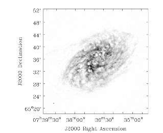
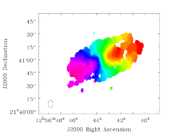
"Other examples of NGC2403 (a moment-0 image of a VLA line dataset) and NGC4826 (a moment-1 image of a BIMA CO line dataset) are shown in the Figure below\n",
"\n",
"\n",
"\n",
"\n",
"\n",
">NGC2403 VLA moment zero (left) and NGC4826 BIMA moment one (right) images as shown in the viewer.\n",
"\n",
"\n",
"**Generating Position-Velocity Diagrams (impv)**\n",
"\n",
"CASA can generate position-velocity (PV) diagrams via the task **impv**:\n",
"\n",
"```\n",
"#impv :: Construct a position-velocity image by choosing two points in the direction plane.\n",
"imagename = '' #Name of the input image\n",
"outfile = '' #Output image name. If empty, no image is written.\n",
"mode = 'coords' #If 'coords', use start and end values. If 'length', use\n",
" #center, length, and pa values.\n",
"width = 1 #Width of slice for averaging pixels perpendicular to the\n",
" #slice. Must be an odd positive integer or valid\n",
" #quantity. See help for details.\n",
"unit = 'arcsec' #Unit for the offset axis in the resulting image. Must be\n",
" #a unit of angular measure.\n",
"chans = '' #Channels to use.\n",
" #Channels must be contiguous. Default is to use all\n",
" #channels.\n",
" region = '' #Region selection. Default is entire image. No selection\n",
" #is permitted in the direction plane.\n",
"\n",
"stokes = 'I' #Stokes planes to use. Planes must be contiguous. Default\n",
" #is to use all stokes.\n",
"mask = [] #Mask to use. Default is none.\n",
" stretch = False #Stretch the mask if necessary and possible? Default False\n",
"```\n",
"\n",
"PV diagrams are generated by \"slicing\" a datacube through the RA/DEC planes. The \"slit\" can be defined either by start/end coordinates or by a length, center coordinate, and position angle. Averaged over the width of the 'slit' the image cube values are then stored in a new image with position and velocity as the two axes. The slit position is specified by a start and end pixel in the RA/DEC plane of the data cube. An angular unit can be set to define what is stored in the resulting PV image.\n",
"\n",
"\n",
"**1-dimensional Smoothing (specsmooth)**\n",
"\n",
"To gain higher signal-to-noise of data cubes, one can smooth the data along one dimension. Typically this is the spectral axis. Hanning and Boxcar smoothing kernels are available in the task **specsmooth**:\n",
"\n",
"```\n",
"#specsmooth :: Smooth an image region in one dimension\n",
"imagename = '' #Name of the input image\n",
"outfile = '' #Output image name.\n",
"region = '' #Region selection. Default is to use the full\n",
" #image.\n",
" box = '' #Rectangular region to select in\n",
" #direction plane. Default is to use the entire\n",
" #direction plane.\n",
"\n",
"mask = '' #Mask to use. Default is none..\n",
"axis = -1 #The profile axis. Default: use the\n",
" #spectral axis if one exists, axis 0\n",
" #otherwise (<0).\n",
"function = 'hanning' #Convolution function. hanning and boxcar\n",
" #are supported functions. Minimum match\n",
" #is supported.\n",
"dmethod = 'copy' #Decimation method. '' means no\n",
" #decimation, 'copy' and 'mean' are also\n",
" #supported (minimum match).\n",
"```\n",
"\n",
"The parameter *dmethod='copy'* allows one to only keep every nth channel, if the smoothing kernel has a width of n. Leaving this parameter empty will return the same size cube as the input and setting it to 'mean' will average planes using the kernel width.\n",
"\n",
"\n",
"**Spectral Line fitting**\n",
"\n",
"**specfit** is a powerful task to perform spectral line fits in data cubes. Three types of fitting functions are currently supported, polynomials, Gaussians, and Lorentzians. **specfit** can fit these functions in two ways: over data that were averaged across a region (*multifit=False*) or on a pixel by pixel basis (*multifit=True*).\n",
"\n",
"```\n",
"#specfit :: Fit 1-dimensional Gaussians and/or polynomial models to an image or image region\n",
"imagename = '' #Name of the input image\n",
"box = '' #Rectangular box in direction coordinate\n",
" #blc, trc. Default: entire image ('').\n",
"region = '' #Region of interest. Default: Do\n",
" #not use a region.\n",
"chans = '' #Channels to use. Channels must be\n",
" #contiguous. Default: all channels ('').\n",
"stokes = '' #Stokes planes to use. Planes must be\n",
" #contiguous. Default: all stokes ('').\n",
"axis = -1 #The profile axis. Default: use the\n",
" #spectral axis if one exists, axis 0\n",
" #otherwise (<0).\n",
"mask = '' #Mask to use. Default is\n",
" #none..\n",
"poly = -1 #Order of polynomial element. Default: do\n",
" #not fit a polynomial (<0).\n",
"estimates = '' #Name of file containing initial estimates.\n",
" #Default: No initial estimates ('').\n",
" ngauss = 1 #Number of Gaussian elements. Default: 1.\n",
" pampest = '' #Initial estimate of PCF profile (gaussian\n",
" #or lorentzian) amplitudes.\n",
" pcenterest = '' #Initial estimate PCF profile centers, in\n",
" #pixels.\n",
" pfwhmest = '' #Initial estimate PCF profile FWHMs, in\n",
" #pixels.\n",
" pfix = '' #PCF profile parameters to fix during fit.\n",
" pfunc = '' #PCF singlet functions to fit. 'gaussian'\n",
" #or 'lorentzian' (minimal match\n",
" #supported). Unspecified means all\n",
" #gaussians.\n",
"\n",
"minpts = 0 #Minimum number of unmasked points\n",
" #necessary to attempt fit.\n",
"multifit = True #If true, fit a profile along the desired\n",
" #axis at each pixel in the specified\n",
" #region. If false, average the non-fit\n",
" #axis pixels and do a single fit to that\n",
" #average profile. Default False.\n",
" amp = '' #Name of amplitude solution image. Default:\n",
" #do not write the image ('').\n",
" amperr = '' #Name of amplitude solution error image.\n",
" #Default: do not write the image ('').\n",
" center = '' #Name of center solution image. Default: do\n",
" #not write the image ('').\n",
" centererr = '' #Name of center solution error image.\n",
" #Default: do not write the image ('').\n",
" fwhm = '' #Name of fwhm solution image. Default: do\n",
" #not write the image ('').\n",
" fwhmerr = '' #Name of fwhm solution error image.\n",
" #Default: do not write the image ('').\n",
" integral = '' #Prefix of name of integral solution image.\n",
" #Name of image will have gaussian\n",
" #component number appended. Default: do\n",
" #not write the image ('').\n",
" integralerr = '' #Prefix of name of integral error solution\n",
" #image. Name of image will have gaussian\n",
" #component number appended. Default: do\n",
" #not write the image ('').\n",
"\n",
"model = '' #Name of model image. Default: do not write\n",
" #the model image ('').\n",
"residual = '' #Name of residual image. Default: do not\n",
" #write the residual image ('').\n",
"wantreturn = True #Should a record summarizing the results be\n",
" #returned?\n",
"logresults = True #Output results to logger?\n",
"gmncomps = 0 #Number of components in each gaussian\n",
" #multiplet to fit\n",
"gmampcon = '' #The amplitude ratio constraints for non-\n",
" #reference components to reference\n",
" #component in gaussian multiplets.\n",
"gmcentercon = '' #The center offset constraints (in pixels)\n",
" #for non-reference components to reference\n",
" #component in gaussian multiplets.\n",
"gmfwhmcon = '' #The FWHM ratio constraints for non-\n",
" #reference components to reference\n",
" #component in gaussian multiplets.\n",
"gmampest = [0.0] #Initial estimate of individual gaussian\n",
" #amplitudes in gaussian multiplets.\n",
"gmcenterest = [0.0] #Initial estimate of individual gaussian\n",
" #centers in gaussian multiplets, in\n",
" #pixels.\n",
"gmfwhmest = [0.0] #Initial estimate of individual gaussian\n",
" #FWHMss in gaussian multiplets, in pixels.\n",
"gmfix = '' #Parameters of individual gaussians in\n",
" #gaussian multiplets to fix during fit.\n",
"logfile = '' #File in which to log results. Default is\n",
" #not to write a logfile.\n",
"goodamprange = [0.0] #Acceptable amplitude solution range. [0.0]\n",
" #=> all amplitude solutions are\n",
" #acceptable.\n",
"goodcenterrange = [0.0] #Acceptable center solution range in pixels\n",
" #relative to region start. [0.0] => all\n",
" #center solutions are acceptable.\n",
"goodfwhmrange = [0.0] #Acceptable FWHM solution range in pixels.\n",
" #[0.0] => all FWHM solutions are\n",
" #acceptable.\n",
"sigma = '' #Standard deviation array or image name.\n",
"```\n",
"\n",
"*Polynomial Fits*\n",
"\n",
"Polynomials can be fit by specifying the polynomial order in *poly*. Negative orders will not fit any polynomials.\n",
"\n",
"*Lorentzian and Gaussian Fits*\n",
"\n",
"Gaussian and Lorentzian fits are very similar, they both require amplitude, center, and FWHM to be fully specified. All of the following discussion is thus valid for both functions. The parameter *pfunc* controls whether Gaussian or Lorentzian functions are to be used. Default is all Gaussians. *pfunc=\\[\\'L\\', \\'G\\', \\'G\\', \\'L\\'\\]* would use Lorentzian, Gaussian, Gaussian, and Lorentzian components in the order they appear in the estimates file (see below).\n",
"\n",
"*One or more single Gaussian/Lorentzian*\n",
"\n",
"For Gaussian and Lorentzian fits, the task will allow multiple components and **specfit** will try to find the best solution. The parameter *space*, however, is usually not uniform and to avoid local minima in the goodness-of-fit space, one can provide initial start values for the fits. This can be done either through the parameters *pampest*, *pcenterest*, and *pfwhmest* for the amplitudes, center, and FWHM estimates in image coordinates. *pfix* can take parameters that specify fixed fit values. Any combination of the characters *'p'* (peak), *'c'* (center), and *'f'* (fwhm) are permitted, e.g. '*fc*' will hold the fwhm and the center constant during the fit. Fixed parameters will have no errors associated with them in the solution. Alternatively, a file with initial values can be supplied by the *estimates* parameter (one Gaussian/Lorentzian parameter set per line). The file has the following format:\n",
"\n",
"```\n",
"[peak intensity], [center], [fwhm], [optional fixed parameter string]\n",
"```\n",
"\n",
"The first three values are required and must be numerical values. The peak intensity must be expressed in map units, while the center and fwhm must be specified in pixels. The fourth value is optional and if present, represents the parameter(s) that should be held constant during the fit (see above). An example estimates file is:\n",
"\n",
"```\n",
" # estimates file indicating that two Gaussians should be fit\n",
" # first guassian estimate, peak=40, center at pixel number 10.5,\n",
" # fwhm = 5.8 pixels, all parameters allowed to vary during\n",
" # fit\n",
" 40, 10.5, 5.8\n",
" # second Gaussian, peak = 4, center at pixel number 90.2,\n",
" # fwhm = 7.2 pixels, hold fwhm constant\n",
" 4, 90.2, 7.2, f\n",
" # end file\n",
"```\n",
"\n",
"and the output of a typical execution, e.g.\n",
"\n",
"```\n",
"specfit(imagename='IRC10216_HC3N.cube_r0.5.image', region='specfit.crtf',\n",
" multifit=F, estimates='', ngauss=2)\n",
"```\n",
"('specfit.crtf' is a CASA regions file, see Section D)\n",
"will be\n",
"\n",
"```\n",
"Fit :\n",
" RA : 09:47:57.49\n",
" Dec : 13.16.46.46\n",
" Stokes : I\n",
" Pixel : [146.002, 164.499, 0.000, *]\n",
" Attempted : YES\n",
" Converged : YES\n",
" Iterations : 28\n",
" Results for component 0:\n",
" Type : GAUSSIAN\n",
" Peak : 5.76 +/- 0.45 mJy/beam\n",
" Center : -15.96 +/- 0.32 km/s\n",
" 40.78 +/- 0.31 pixel\n",
" FWHM : 7.70 +/- 0.77 km/s\n",
" 7.48 +/- 0.74 pixel\n",
" Integral : 47.2 +/- 6.0 mJy/beam.km/s\n",
" Results for component 1:\n",
" Type : GAUSSIAN\n",
" Peak : 4.37 +/- 0.33 mJy/beam\n",
" Center : -33.51 +/- 0.58 km/s\n",
" 23.73 +/- 0.57 pixel\n",
" FWHM : 15.1 +/- 1.5 km/s\n",
" 14.7 +/- 1.5 pixel\n",
" Integral : 70.2 +/- 8.8 mJy/beam.km/s\n",
"```\n",
"\n",
"If *wantreturn=True* (the default value), the task returns a python dictionary (here captured in a variable with the inventive name of '*fitresults'*) :\n",
"\n",
"```\n",
"fitresults=specfit(imagename='IRC10216_HC3N.cube_r0.5.image', region='specfit.rgn', multifit=F, estimates='', ngauss=2)\n",
"```\n",
"\n",
"The values can then be used by other python code for further processing.\n",
"\n",
"*Gaussian Multiplets*\n",
"\n",
"It is possible to fit a number of Gaussians together, as multiplets with restrictions. All restrictions are relative to a reference Gaussian (the zero'th component of each multiplet). *gncomps* specifies the number of Gaussians for each multiplets, and, in fact, a number of these multiplets can be fit simultaneously. *gncomps=\\[2,4,3\\]*, e.g. fits a 2-component Gaussian, a 4-component Gaussian, and a 3-component Gaussian all at once. The initial parameter estimates can be specified with the *gmampest*, *gmcenterest*, and *gmfwhmest* parameters and the estimates are simply listed in the sequence of *gncomps*. E.g. if *gncomps=\\[2,4,3\\]* is specified with multiplet G0 consisting of 2 Gaussians a, b, multiplet G1 of 4 Gaussians c, d, e, f, and multiplet G2 of three Gaussians g, h, i, the parameter list in *gm\\*est* would be like *gm\\*est=\\[a,b,c,d,e,f,g,h,i\\]*.Restrictions can be specified via the *gmampcon* parameter for the amplitude ratio (non-reference to reference), *gmcentercon* for the offset in pixels (to a reference), and *gmfwhmcon* for the FWHM ratio (non-reference to reference). A value of 0 will not constrain anything. The reference is always the zero'th component in each multiplet, in our example, Gaussians a, c, and g. They cannot be constrained. So *gmncomps=\\[2, 4, 3\\]*, *gmampcon= \\[ 0 , 0.2, 0 , 0.1, 4.5, 0 \\]*, *gcentercon=\\[24.2, 45.6, 92.7, 0 , -22.8, -33.5\\],* and *gfwhmcon=\\' \\'* would constrain Gaussians b relative to a with a 24.2 pixel offset, Gaussian d to c with a amplitude ratio of 0.2 and a 45.6 pixel offset, Gaussian e to c with a offset of 92.7 pixels, etc. Restrictions will overrule any estimates.The parameters *goodamprange*, *goodcenterrange*, and *goodfwhmrange* can be used to limit the range of amplitude, center, and fwhm solutions for all Gaussians.\n",
"\n",
"*Pixel-by-pixel fits*\n",
"\n",
"As mentioned above, **specfit** can also fit spectral cubes on a pixel by pixel basis. In this case, one can choose to write none, any or all of the solution and error images for Gaussian/Lorentzian fits via the parameters *amp*, *amperr*, *center*, *centererr*, *fwhm*, and *fwhmerr*. Each Gaussian component will produce a set of images *\\_0, \\_1*, etc. suffixes. Writing analogous images for polynomial coefficients is not yet supported although polynomial fits when *multifit=True* is supported. Best fit coefficients are written to the logger. Pixels for which fits were not attempted or did not converge will be masked as bad.\n",
"\n",
"**Spatial Spectral Line Properties**\n",
"\n",
"**specflux** calculates the flux as a function of frequency and velocity over a selected spatial region. Flux densities of Jy/beam are being converted to Jy by properly integrating over the selected region.The input parameters of **specflux** are:\n",
"\n",
"```\n",
"#specflux :: Report details of an image spectrum.\n",
"imagename = '' #Name of the input image\n",
"box = '' #Rectangular region to select in\n",
" #direction plane. Default is to use the entire\n",
" #direction plane.\n",
" region = '' #Region selection. Default is to use the full\n",
" #image.\n",
"\n",
"chans = '' #Channels to use. Default is to use all\n",
" #channels.\n",
"stokes = '' #Stokes planes to use. Default is to\n",
" #use all Stokes planes.\n",
"mask = '' #Mask to use. Default\n",
" #is none.\n",
"unit = 'km/s' #Unit to use for the abscissa. Must be\n",
" #conformant with a typical spectral axis\n",
" #unit.\n",
"major = '' #Major axis of overriding restoring beam.\n",
" #If specified, must be a valid quantity.\n",
"minor = '' #Minor axis of overriding restoring beam.\n",
" #If specified, must be a valid quantity\n",
"logfile = '' #File which to write details. Default is\n",
" #to not write to a file.\n",
"```\n",
"\n",
"The results can be written into a logfile to be plotted in other packages.\n",
"\n",
"**Plot Spectra on a Map (plotprofilemap)**\n",
"\n",
"The **profilemap** task enables plotting spectra according to their pointing directions (a.k.a. a profile map) in plots. The input should be CASA image,or FITS format cube. Spectra within the cube are averaged into a bin number specified with the *numpanels* keyword. Absent or masked data are treated according to *plotmasked* keyword setting.\n",
"\n",
"```\n",
"plotprofilemap(imagename='interesting_spectralcube_casaimge.im',\n",
"figfile = 'grid_map.png',\n",
"separatepanel=F,\n",
"spectralaxis = 'velocity',\n",
"title = 'myprofilemap',\n",
"transparent = F,\n",
"showaxislabel = True,\n",
"showtick = True,\n",
"showticklabel = True,\n",
"pol=0,\n",
"numpanels='8')\n",
"```\n",
"\n",
"**Calculation of Rotation Measures**\n",
"\n",
"**rmfit** is an image domain task that accepts an input cube image containing Stokes Q and U axes and will generate the rotation measure by performing a least square fit in the image domain to obtain the best fit to the equation $\\chi = \\chi_0 + RM\\times \\lambda^2$.\n",
"\n",
"The inputs to **rmfit** are:\n",
"\n",
"```\n",
"#rmfit :: Calculate rotation measure.\n",
"imagename = '' #Name(s) of the input image(s). Must be specified.\n",
"rm = '' #Output rotation measure image name. If not specified, no\n",
" #image is written.\n",
"rmerr = '' #Output rotation measure error image name. If not\n",
" #specified, no image is written.\n",
"pa0 = '' #Output position angle (degrees) at zero wavelength image\n",
" #name. If not specified, no image is written.\n",
"pa0err = '' #Output position angle (degrees) at zero wavelength error\n",
" #image name. If not specified, no image is written.\n",
"nturns = '' #Output number of turns image name. If not specified, no\n",
" #image is written.\n",
"chisq = '' #Output reduced chi squared image name. If not specified,\n",
" #no image is written.\n",
"sigma = '' #Estimate of the thermal noise. A value less than 0 means\n",
" #auto estimate.\n",
"rmfg = 0.0 #Foreground rotation measure in rad/m/m to subtract.\n",
"rmmax = 0.0 #Maximum rotation measure in rad/m/m for which to solve.\n",
" #IMPORTANT TO SPECIFY.\n",
"maxpaerr = 1e+30 #Maximum input position angle error in degrees to allow in\n",
" #solution determination.\n",
"```\n",
"\n",
"This task generates the rotation measure image from stokes Q and U measurements at several different frequencies. You are required to specify the name of at least one image with a polarization axis containing stokes Q and U planes and with a frequency axis containing more than two pixels. The frequencies do not have to be equally spaced (i.e. the frequency coordinate can be a tabular coordinate). It will work out the position angle images for you. You may also specify multiple image names, in which case these images will first be concatenated along the spectral axis using **ia.imageconcat**. The requirements are that for all images, the axis order must be the same and the number of pixels along each axis must be identical, except for the spectral axis which may differ in length between images. The spectral axis need not be contiguous from one image to another. See also the i**magepol.fourierrotationmeasure** function for a new Fourier-based approach.Rotation measure algorithms that work robustly are few. The main problem is in trying to account for the $n- \\pi$ ambiguity (see Leahy et al.1986 - Appendix A.1) [\\[1\\]](#Bibliography) and the [MIRIAD manual](http://www.cfa.harvard.edu/sma/miriad/manuals/SMAuguide/smauserhtml/imrm.html).\n",
"\n",
"But as in all these algorithms, the basic process is that for each spatial pixel, the position angle vs frequency data is fit to determine the rotation measure and the position angle at zero wavelength (and associated errors). An image containing the number of $n- \\pi$ turns that were added to the data at each spatial pixel and for which the best fit was found can be written. The reduced $\\chi^2$ image for the fits can also be written. Any combination of output images can be written.\n",
"\n",
"\n",
"**NOTE**: No assessment of curvature (i.e. deviation from the simple linear position angle - $lambda^2$ functional form) is made.\n",
"
\n",
"\n",
"The parameter *sigma* gives the thermal noise in Stokes Q and U. By default it is determined automatically using the image data. But if it proves to be inaccurate (maybe not many signal-free pixels), it may be specified. This is used for calculating the error in the position angles (via propagation of Gaussian errors).The argument *maxpaerr* specifies the maximum allowable error in the position angle that is acceptable. The default is an infinite value. From the standard propagation of errors, the error in the linearly polarized position angle is determined from the Stokes Q and U images (at each directional pixel for each frequency). If the position angle error for any pixel exceeds the specified value, the position angle at that pixel is omitted from the fit. The process generates an error for the fit and this is used to compute the errors in the output images.\n",
"\n",
"\n",
"**NOTE**: *maxpaerr* is not used to mask pixels in the output images.\n",
"
\n",
"\n",
"The argument *rmfg* is used to specify a foreground RM value. For example, you may know the mean RM in some direction out of the Galaxy, then including this can improve the algorithm by reducing ambiguity. The parameter *rmmax* specifies the maximum absolute RM value that should be solved for. This quite an important parameter. If you leave it at the default, zero, no ambiguity handling will be used. So some a priori information should be supplied; this is the basic problem with rotation measure algorithms.\n",
"\n",
"\n",
"\n"
]
},
{
"cell_type": "markdown",
"metadata": {
"id": "3TbvveRNkunr"
},
"source": [
"**Calculation of Spectral Indices and Higher Order Polynomials**\n",
"\n",
"This application fits a power logarithmic polynomial or a logarithmic transformed polynomial to pixel values along a specified axis of an image or images. These functions are most often used for fitting the spectral index and higher order terms of a spectrum. A power logarithmic polynomial has the form\n",
"\n",
"$y = \\frac{c_0 x}{D^{(c_1 + c_2 \\ln(x/D) + c_3 \\ln(x/D)^2 + c_n \\ln(x/D)^{(n - 1)})}}$\n",
"\n",
"and a logarithmic transformed polynomial is simply the result of this equation after taking the natural log of both sides so that it has the form\n",
"\n",
"$\\ln(y) = c_0 + c_1 \\ln(x) + c_2 \\ln(x/D)^2 + ... + c_n \\ln(x/D)^n$\n",
"\n",
"Because the logarithm of the ordinate values must be taken before fitting a logarithmic transformed polynomial, all non-positive pixel values are effectively masked for the purposes of fitting. The coefficients of the two forms are equal to each other except that c0 in the second equation is equal to $\\ln(c_0)$ of the first. In the case of fitting a spectral index, which is traditionally represented as $\\alpha$, is equal to $c_1$. In both cases, $D$ is a normalization constant used so that abscissa values are closer to unity when they are sent to the fitter. This generally improves the probability that the fit will converge. This parameter may be specified via the *div* parameter. A value of 0 (the default) indicates that the application should determine a reasonable value for $D$, which is determined via$D = 10^{\\int(\\log10(\\sqrt(\\min(x)*\\max(x)))}$where *min(x)* and *max(x)* are the minimum and maximum abscissa values, respectively.The inputs are:\n",
"\n",
"```\n",
" #spxfit :: Fit a 1-dimensional model to an image or image region\n",
"for determination of spectral index.\n",
"imagename = #Name of the input image(s)\n",
"box = '' #Rectangular box in\n",
" #direction coordinate blc, trc.\n",
" #Default: entire image ('').\n",
"region = '' #Region of interest. Default:\n",
" #Do not use a region.\n",
"chans = '' #Channels to use. Channels\n",
" #must be contiguous. Default: all channels ('').\n",
"stokes = '' #Stokes planes to\n",
" #use. Planes must be contiguous. Default:\n",
" #all stokes ('').\n",
"axis = -1 #The profile axis. Default:\n",
" #use the spectral axis if one\n",
" #exists, axis 0 otherwise (<0).\n",
"mask = '' #Mask to use. Default is none.\n",
"minpts = 1 #Minimum number of unmasked\n",
" #points necessary to attempt\n",
" #fit.\n",
"multifit = True #If true, fit a profile\n",
" #along the desired axis at each\n",
" #pixel in the specified\n",
" #region. If false, average the\n",
" #non-fit axis pixels and do\n",
" #a single fit to that average\n",
" #profile. Default False.\n",
" spxsol = '' #Name of the spectral index\n",
" #function coefficient solution\n",
" #image to write.\n",
" spxerr = '' #Name of the spectral index\n",
" #function coefficient error\n",
" #image to write.\n",
" model = '' #Name of model\n",
" #image. Default: do not write the model\n",
" #image ('').\n",
" residual = '' #Name of residual\n",
" #image. Default: do not write the\n",
" #residual image ('').\n",
"spxtype = 'plp' #Type of function to\n",
" #fit. 'plp' => power logarithmic\n",
" #polynomial, 'ltp' =>\n",
" #logarithmic transformed polynomial.\n",
"spxest = [] #Initial estimates for the\n",
" #spectral index function\n",
" #coefficients.\n",
"spxfix = [] #Fix the corresponding spectral index function\n",
" #coefficients during the fit. True=>hold fixed.\n",
"div = 0 #Divisor (numerical value or\n",
" #quantity) to use in the\n",
" #logarithmic terms of the\n",
" #plp or ltp function. 0 =>\n",
" #calculate a useful value on the fly.\n",
"wantreturn = True #Should a record summarizing\n",
" #the results be returned?\n",
"logresults = True #Output results to logger?\n",
"logfile = '' #File in which to log\n",
" #results. Default is not to write a\n",
" #logfile.\n",
"sigma = -1 #Standard deviation array or image name(s).\n",
" outsigma = '' #Name of output image used\n",
" #for standard deviation. Ignored\n",
" #if sigma is empty.\n",
"```\n",
"\n",
"For more than a single input image or cube, all images must have the same dimensions along all axes other than the fit axis. *multifit* will perform a per-pixel fit, otherwise there will be a single value over the entire region.\n",
"\n",
"\n",
"**Search for Spectral Line Rest Frequencies**\n",
"\n",
"The **slsearch** task allows the spectral line enthusiast to find their favorite spectral lines in subset of the [Splatalogue spectral line catalog](http://www.splatalogue.net) which is distributed with CASA. In addition, one can export custom catalogs from Splatalogue and import them to CASA using the task **splattotable** (next section) or tool method **sl.splattotable**. One can even import catalogs with lines not in Splatalogue using the same file format.The inputs to **slsearch** are as follows:\n",
"\n",
"```\n",
"#slsearch :: Search a spectral line table.\n",
"tablename = '' #Input spectral line table name to\n",
" #search. If not specified, use the\n",
" #default table in the system.\n",
"outfile = '' #Results table name. Blank means do not\n",
" #write the table to disk.\n",
"freqrange = [84, 90] #Frequency range in GHz.\n",
"species = [''] #Species to search for.\n",
"reconly = False #List only NRAO recommended\n",
" #frequencies.\n",
"chemnames = [''] #Chemical names to search for.\n",
"qns = [''] #Resolved quantum numbers to search\n",
" #for.\n",
"rrlinclude = True #Include RRLs in the result set?\n",
"rrlonly = False #Include only RRLs in the result set?\n",
" intensity = -1 #CDMS/JPL intensity range. -1 -> do not\n",
" #use an intensity range.\n",
" smu2 = -1 #S*mu*mu range in Debye**2. -1 -> do\n",
" #not use an S*mu*mu range.\n",
" loga = -1 #log(A) (Einstein coefficient) range.\n",
" #-1 -> do not use a loga range.\n",
" eu = -1 #Upper energy state range in Kelvin. -1\n",
" #-> do not use an eu range.\n",
" el = -1 #Lower energy state range in Kelvin. -1\n",
" #-> do not use an el range.\n",
"\n",
"verbose = True #List result set to logger (and\n",
" #optionally logfile)?\n",
" logfile = '' #List result set to this logfile (only\n",
" #used if verbose=True).\n",
" append = True #If true, append to logfile if it\n",
" #already exists, if false overwrite\n",
" #logfile if it exists. Only used if\n",
" #verbose=True and logfile not blank.\n",
"\n",
"wantreturn = True #If true, return the spectralline tool\n",
" #associated with the result set.\n",
"```\n",
"\n",
"The table is provided in the *tablename* parameter but if it is blank (the default), the catalog which is included with CASA will be used. Searches can be made in a parameter space with large dimensionality:\n",
"\n",
"```\n",
"freqrange Frequency range in GHz. \n",
"species Species to search for. \n",
"reconly List only NRAO recommended frequencies.\n",
"chemnames Chemical names to search for. \n",
"qns Resolved quantum numbers to search for. \n",
"intensit CDMS/JPL intensity range. \n",
"smu2 $S\\mu^{2}$ range in Debye$^2$. \n",
"loga log(A) (Einstein coefficient) range. \n",
"el Lower energy state range in Kelvin. \n",
"eu Upper energy state range in Kelvin. \n",
"rrlinclude Include RRLs in the result set? \n",
"rrlonly Include only RRLs in the result set?\n",
"```\n",
"\n",
"Notation is as found in the Splatalogue catalog.\n",
"\n",
"Example: Search for all lines of the species HOCN and HOCO$^+$ in the 200-300GHz range:\n",
"\n",
"```\n",
"slsearch(outfile='myresults.tbl', freqrange = [200,300],\n",
" species=['HOCN', 'HOCO+'])\n",
"```\n",
"\n",
"The task can also return a python dictionary if assigned a variable like:\n",
"\n",
"```\n",
"myLines = slsearch(outfile='myresults.tbl', freqrange = [200,300],\n",
" species=['HOCN', 'HOCO+'])\n",
"```\n",
"\n",
"\n",
"**Convert Exported Splatalogue Catalogs to CASA Tables**\n",
"\n",
"In some cases, the internal spectral line catalog may not contain the lines in which one is interested. In that case, one can export a catalog from [Splatalogue](http://www.splatalogue.net) or even create their own \\'by hand\\' (be careful to get the format exactly right though!). CASA's task **splattotable** can then be used to create a CASA table that contains these lines and can be searched:\n",
"\n",
"```\n",
"#splattotable :: Convert a downloaded Splatalogue spectral line list to a casa table.\n",
"filenames = [''] #Files containing Splatalogue lists.\n",
"table = '' #Output table name.\n",
"wantreturn = True #Do you want the task to return a spectralline tool attached to the results table?\n",
"```\n",
"\n",
"A search in Splatalogue will return a catalog that can be saved in a file (look for the \\'Export\\' section after the results on the search results page). The exported filename(s) should be entered in the *filenames* parameter of **splattotable**. The downloaded files must be in a specific format for this task to succeed. If you use the Splatalogue *Export CASA fields* feature, you should have no difficulties.\n",
"\n",
"\n",
"### Bibliography\n",
"\n",
"1. Leahy, J.P., Pooley, G.G., & Jagers, W.J. 1986, A&A, 156, 234 (http://adsabs.harvard.edu/abs/1986A%26A...156..234L)\n",
"\n",
"\n",
"***\n",
"\n",
"\n",
"\n",
"\n",
"\n",
"\n"
]
},
{
"cell_type": "markdown",
"metadata": {
"id": "cxF8UvFbkunt"
},
"source": [
"## Image Plane Analysis\n",
"\n",
"**Image-plane Component Fitting**\n",
"\n",
"Task **imfit** inputs are:\n",
"\n",
"```\n",
"#imfit :: Fit one or more elliptical Gaussian components on an image region(s)\n",
"imagename = '' #Name of the input image\n",
"box = '' #Specify one or more box regions for the fit.\n",
"region = '' #Region.\n",
"chans = '' #Spectral channels on which to perform fit.\n",
"stokes = '' #Stokes parameter to fit. If blank, first stokes plane is\n",
" #used.\n",
"mask = '' #Mask to use. Default is none.\n",
"includepix = [] #Range of pixel values to include for fitting.\n",
"excludepix = [] #Range of pixel values to exclude for fitting.\n",
"residual = '' #Name of output residual image.\n",
"model = '' #Name of output model image.\n",
"estimates = '' #Name of file containing initial estimates of component\n",
" #parameters.\n",
"logfile = '' #Name of file to write fit results.\n",
"newestimates = '' #File to write fit results which can be used as initial\n",
" #estimates for next run.\n",
"complist = '' #Name of output component list table.\n",
"dooff = False #Also fit a zero level offset? Default is False\n",
"rms = -1 #RMS to use in calculation of uncertainties. Numeric or\n",
" #valid quantity (record or string). If numeric, it is\n",
" #given units of the input image. If quantity, units must\n",
" #conform to image units. If not positive, the rms of the\n",
" #residual image, in the region of the fit, is used.\n",
"noisefwhm = '' #Noise correlation beam FWHM. If numeric value,\n",
" #interpreted as pixel widths. If quantity (dictionary,\n",
" #string), it must have angular units.\n",
"```\n",
"\n",
"**imfit** will return (as a Python dictionary) the results of the fit, but the results can also be written into a component list table or a logfile.\n",
"\n",
"\n",
"**NOTE**: To fit more than a single component, you must provide starting estimates for each component via the *estimates* file. See ''*help imfit'*' for more details on this. A noise estimate will be calculated automatically or can be provided through the *rms* and *noisefwhm* keywords.\n",
"
\n",
"\n",
"\n",
"*Examples for imfit*\n",
"\n",
"```\n",
"#First fit only a single component at a time\n",
"#This is OK since the components are well-separated and not blended\n",
"#Box around component A\n",
"xfit_A_res = imfit('b1608.demo.clean2.image',box='121,121,136,136',\n",
" newestimates='b1608.demo.clean2.newestimate')\n",
"\n",
"#Now extract the fit part of the return value\n",
"xfit_A = xfit_A_res['results']['component0']\n",
"#xfit_A\n",
"#Out[7]:\n",
"#{'flux': {'error': array([ 6.73398035e-05, 0.00000000e+00, 0.00000000e+00,\n",
"#0.00000000e+00]),\n",
"#'polarisation': 'Stokes',\n",
"#'unit': 'Jy',\n",
"#'value': array([ 0.01753742, 0. , 0. , 0. ])},\n",
"#'label': '',\n",
"#'shape': {'direction': {'error': {'latitude': {'unit': 'arcsec',\n",
"#'value': 0.00041154866279462775},\n",
"#'longitude': {'unit': 'arcsec',\n",
"#'value': 0.00046695916589535109}},\n",
"#'m0': {'unit': 'rad', 'value': -2.0541102061078207}, NOTE: 'm0' and 'm1' are the coordinates of peak/controid\n",
"#'m1': {'unit': 'rad', 'value': 1.1439131060384089}, NOTE: 'm0' and 'm1' are the coordinates of peak/controid\n",
"#'refer': 'J2000',\n",
"#'type': 'direction'},\n",
"#'majoraxis': {'unit': 'arcsec', 'value': 0.29100166137741568},\n",
"#'majoraxiserror': {'unit': 'arcsec',\n",
"#'value': 0.0011186420613222663},\n",
"#'minoraxis': {'unit': 'arcsec', 'value': 0.24738110059830495},\n",
"#'minoraxiserror': {'unit': 'arcsec',\n",
"#'value': 0.0013431999725066338},\n",
"#'positionangle': {'unit': 'deg', 'value': 19.369249322401796},\n",
"#'positionangleerror': {'unit': 'rad',\n",
"#'value': 0.016663189295782171},\n",
"#'type': 'Gaussian'},\n",
"#'spectrum': {'frequency': {'m0': {'unit': 'GHz', 'value': 1.0},\n",
"#'refer': 'LSRK',\n",
"#'type': 'frequency'},\n",
"#'type': 'Constant'}}\n",
"\n",
"#Now the other components\n",
"xfit_B_res = imfit('b1608.demo.clean2.image',box='108,114,120,126',\n",
" newestimates='b1608.demo.clean2.newestimate',append=True)\n",
"xfit_B = xfit_B_res['results']['component0']\n",
"\n",
"xfit_C_res= imfit('b1608.demo.clean2.image',box='108,84,120,96')\n",
"xfit_C = xfit_C_res['results']['component0']\n",
"\n",
"xfit_D_res = imfit('b1608.demo.clean2.image',box='144,98,157,110')\n",
"xfit_D = xfit_D_res['results']['component0']\n",
"\n",
"print \"\"\n",
"print \"Imfit Results:\"\n",
"print \"--------------\"\n",
"print \"A Flux = %6.4f Bmaj = %6.4f\" % (xfit_A['flux']['value'][0],xfit_A['shape']['majoraxis']['value'])\n",
"print \"B Flux = %6.4f Bmaj = %6.4f\" % (xfit_B['flux']['value'][0],xfit_B['shape']['majoraxis']['value'])\n",
"print \"C Flux = %6.4f Bmaj = %6.4f\" % (xfit_C['flux']['value'][0],xfit_C['shape']['majoraxis']['value'])\n",
"print \"D Flux = %6.4f Bmaj = %6.4f\" % (xfit_D['flux']['value'][0],xfit_D['shape']['majoraxis']['value'])\n",
"print \"\"\n",
"```\n",
"\n",
"Now try fitting four components together. For this we will have to provide an estimate file. We will use the clean beam for the estimate of the component sizes:\n",
"\n",
"```\n",
"estfile=open('b1608.demo.clean2.estimate','w')\n",
"print >>estfile,'#peak, x, y, bmaj, bmin, bpa'\n",
"print >>estfile,'0.017, 128, 129, 0.293arcsec, 0.238arcsec, 21.7deg'\n",
"print >>estfile,'0.008, 113, 120, 0.293arcsec, 0.238arcsec, 21.7deg'\n",
"print >>estfile,'0.008, 113, 90, 0.293arcsec, 0.238arcsec, 21.7deg'\n",
"print >>estfile,'0.002, 151, 104, 0.293arcsec, 0.238arcsec, 21.7deg'\n",
"estfile.close()\n",
"```\n",
"\n",
"Then, this can be used in **imfit**:\n",
"\n",
"```\n",
"fit_all_res = imfit('b1608.demo.clean2.image',\n",
" estimates='b1608.demo.clean2.estimate',\n",
" logfile='b1608.demo.clean2.imfitall.log',\n",
" newestimates='b1608.demo.clean2.newestimate',\n",
" box='121,121,136,136,108,114,120,126,108,84,120,96,144,98,157,110')\n",
"#Now extract the fit part of the return values\n",
"xfit_allA = xfit_all_res['results']['component0']\n",
"xfit_allB = xfit_all_res['results']['component1']\n",
"xfit_allC = xfit_all_res['results']['component2']\n",
"xfit_allD = xfit_all_res['results']['component3']\n",
"```\n",
"\n",
"These results are almost identical to those from the individual fits. You can see a nicer printout of the fit results in the logfile.\n",
"\n",
"\n",
"**2-dimensional Smoothing; Image Convolution**\n",
"\n",
"A data cube can be smoothed across spatial dimensions with **imsmooth**. The inputs are:\n",
"\n",
"```\n",
"#imsmooth :: Smooth an image or portion of an image\n",
"imagename = '' #Name of the input image. Must be\n",
" #specified.\n",
"kernel = 'gauss' #Type of kernel to use. Acceptable values\n",
" #are 'b', 'box', or 'boxcar' for a\n",
" #boxcar kernel, 'g', 'gauss', or\n",
" #'gaussian' for a gaussian kernel, 'c',\n",
" #'common', or 'commonbeam' to use the\n",
" #common beam of an image with multiple\n",
" #beams as the gaussian to which to\n",
" #convolve all the planes, 'i' or 'image'\n",
" #to use an image as the kernel.\n",
" beam = '' #Alternate way of describing a Gaussian.\n",
" #If specified, must be a dictionary with\n",
" #keys 'major', 'minor', and 'pa' (or\n",
" #'positionangle'). Do not specify beam\n",
" #if specifying major, minor, and pa.\n",
" #Example: Example: {'major': '5arcsec',\n",
" #'minor': '2arcsec', 'pa': '20deg'}.\n",
" targetres = False #If gaussian kernel, specified parameters\n",
" #are to be resolution of output image\n",
" #(True) or parameters of gaussian to\n",
" #convolve with input image (False).\n",
" major = '' #Major axis for the kernels. Standard\n",
" #quantity representation. Must be\n",
" #specified for kernel='boxcar'. Example:\n",
" #'4arcsec'.\n",
" minor = '' #Minor axis. Standard quantity\n",
" #representation. Must be specified for\n",
" #kernel='boxcar'. Example: '2arcsec'.\n",
" pa = '' #Position angle used only for gaussian\n",
" #kernel. Standard quantity\n",
" #representation. Example: '40deg'.\n",
"\n",
"region = '' #Region selection. See Default is to use the full\n",
" #image.\n",
"box = '' #Rectangular region to select in\n",
" #direction plane. Default is to use the entire\n",
" #direction plane.\n",
"chans = '' #Channels to use. Default is to use all\n",
" #channels.\n",
"stokes = '' #Stokes planes to use. Default is to\n",
" #use all Stokes planes.\n",
"mask = '' #Mask to use. Default\n",
" #is none.\n",
"outfile = '' #Output image name. Must be specified.\n",
"overwrite = False #Overwrite (unprompted) pre-existing\n",
" #output file?\n",
"```\n",
"\n",
"where the cube/image imagename will be convolved with a kernel defined in the *kernel* keyword. Kernels *'gauss'* and *'boxcar'* need the major and minor axes sizes as input, the Gaussian kernel smoothing also requires a position angle. By default, the kernel size defines the kernel itself, i.e. the data will be smoothed with this *kernel*. If the *targetres* parameter for Gaussian kernels is set to *'True'*, major and minor axes will be those from the output resolution, and the kernel will be adjusted for each plane to arrive at the final resolution. The 'commonbeam' kernel is to be used when the beam shape is different as a function of frequency. This option will then smooth all planes to a single beam, defined by the largest beam in the cube. With the *'image'* kernel, one can specify an image that will serve as the convolution kernel. A scale factor can be applied, which defaults to flux conservation where units are Jy/beam or Jy/beam.km/s. For all other units, like K, the output will be scaled by the inverse of the convolution kernel. e.g., in the extreme case of a flat distribution the values before and after smoothing will be the same.\n",
"\n",
"Examples:\n",
"\n",
"1) Smoothing with a Gaussian kernel 20\" by 10\"\n",
"\n",
"```\n",
"imsmooth( imagename='my.image', kernel='gauss', major='20arcsec', minor='10arcsec',targetres=T)\n",
"```\n",
"\n",
"2\\) Smoothing using pixel coordinates and a boxcar kernel.\n",
"\n",
"```\n",
"imsmooth( imagename='new.image', major='20pix', minor='10pix', kernel='boxcar')\n",
"```\n",
"\n",
"***\n",
"\n",
"\n",
"\n",
"\n",
"\n",
"\n",
"\n"
]
},
{
"cell_type": "markdown",
"metadata": {
"id": "UIggdMzgkunw"
},
"source": [
"## Math Operations / Statistics\n",
"\n",
"Mathematical operations on images are typically completed using the CASA task [immath](../api/casatasks.rst#analysis), and image statistics may be derived using the CASA tasks [imstat](../api/casatasks.rst#analysis) and [imdev](../api/casatasks.rst#analysis). Here, we give an overview of how these tasks are used.\n",
"\n",
"**Mathematical Operations on Images**\n",
"\n",
"The CASA task **immath** is useful for performing mathematical operations on images and on specific channels within images, including e.g. addition or subtraction of two cubes, squaring an image, computing a spectral index, and determining polarization angles and intensities. The inputs are:\n",
"\n",
"```\n",
"#immath :: Perform math operations on images\n",
"imagename = '' #a list of input images\n",
"mode = 'evalexpr' #mode for math operation (evalexpr, spix, pola, poli)\n",
" expr = '' #Mathematical expression using images\n",
" varnames = '' #a list of variable names to use with the image files\n",
"\n",
"outfile = 'immath_results.im' #File where the output is saved\n",
"mask = '' #Mask to use. Default is none.\n",
"region = '' #Region selection.\n",
" #Default is to use the full image.\n",
"box = '' #Rectangular region to\n",
" #select in direction plane.\n",
" #Default is to use the\n",
" #entire direction plane.\n",
"chans = '' #Channels to use.\n",
" #Default is to use all channels.\n",
"stokes = '' #Stokes planes to use.\n",
" #Default is to use all Stokes planes.\n",
"imagemd = '' #An image name from which metadata should be copied. The input\n",
" #can be either an image listed under imagename or any other\n",
" #image on disk. Leaving this parameter unset may copy header\n",
" #metadata from any of the input images, which\n",
" #one is not guaranteed.\n",
"```\n",
"\n",
"\n",
"**Alert:** **immath** does not convert any brightness units, e.g. from Jy/beam to K or vice versa. The user is responsible for making sure the images are consistent with the values in the header and the image. It is not advisable to mix input images that are in different units or have different beam sizes.\n",
"
\n",
"\n",
"The *imagename* parameter must be given the name of a single image as a string (e.g. *imagename='image1.im'*) or the names of multiple images in a list of strings (e.g. *imagename=\\['image1.im', 'image2.im'\\]* ). The **immath** task outputs an image file, and the name of the output file is specified using the *outfile* parameter.\n",
"\n",
"The *mode* parameter selects what **immath** is to do. The default, *mode='evalexpr'*, allows the user to specify a mathematical operation to execute on the input images through the *expr* sub-parameter. The mathematical expression is specified in *expr* as a Lattice Expression Language (LEL) string (see the [page on LEL strings](image_analysis.ipynb#lattice-expression-language)). The standard usage for *mode='evalexpr'* is to input a list of images into the *imagename* parameter, and then refer to them in the *expr* subparameter in LEL by the names IM0, IM1, \\.... For example,\n",
"\n",
"```\n",
"immath(imagename=['image1.im','image2.im'],expr='IM0-IM1',outfile='ImageDiff.im')\n",
"```\n",
"\n",
"would subtract the second image given from the first.\n",
"\n",
"For the special modes *'spix'*, *'pola'*, and *'poli'*, the images required for the operation may need to be listed in *imagename* in a particular order. See examples of usage for polarization data below, paying particular attention to posted alerts.\n",
"\n",
"The mathematical expression can be computed on the entire image cube, or on selected regions and image planes, which can be specified through the *mask*, *region*, *box*, *chans*, and *stokes* parameters. Mask specification is done using the *mask* parameter which can optionally contain an on-the-fly mask expression (in [LEL](image_analysis.ipynb#lattice-expression-language)) or point to an image with a pixel mask. In some cases, one may like to use a flat image (e.g. a moment image) mask applied to an entire cube. The *stretch=True* subparameter in *mask* allows one to expand the mask to all planes (i.e. channels or Stokes planes) of the cube. Region selection can also be carried out through the *region* parameter (see the pages on [Region Files](image_analysis.ipynb#region-files) and [Region File Format](image_analysis.ipynb#region-file-format)) and *box* parameter, while image plane selection is controlled by *chans* and *stokes* parameters.\n",
"\n",
"The image metadata in the output file is adopted from another image, which can be specified through the *imagemd* parameter. In *imagemd*, input the name of the image from which the metadata should be copied and used for the output image. If left blank, the task may pick any of the input image headers, so it is better to define this parameter. In fact, the image specified in *imagemd* can be any image, even an image that is not part of the calculations in **immath**.\n",
"\n",
"Detailed examples of **immath** usage are given below.\n",
"\n",
"*Examples for immath*\n",
"\n",
"In the following, we show a examples of **immath** usage. Note that the image names in the *expr* are assumed to refer to existing image files in the current working directory.\n",
"\n",
"- Simple math - Select a single plane (channel 22) of the 3-D cube:\n",
"\n",
"```\n",
"immath(imagename='ngc5921.demo.cleanimg.image',\n",
" expr='IM0',chans='22',\n",
" outfile='ngc5921.demo.chan22.image')\n",
"```\n",
"\n",
"Double all values in our image:\n",
"\n",
"```\n",
"immath(imagename=['ngc5921.demo.chan22.image'],\n",
" expr='IM0*2.0',\n",
" outfile='ngc5921.demo.chan22double.image' )\n",
"```\n",
"\n",
"Square all values in our image:\n",
"\n",
"```\n",
"immath(imagename=['ngc5921.demo.chan22.image'],\n",
" expr='IM0^2',\n",
" outfile='ngc5921.demo.chan22squared.image' )\n",
"```\n",
"\n",
"\n",
"**NOTE**: The units in the output image are still claimed to be \"Jy/beam\", i.e. **immath** will not correctly scale the units in the image for non-linear cases like this. Beware!\n",
"
\n",
"\n",
"Subtract our image containing channel 22 from the original 3-D cube. Note that in this example, the 2-D plane (channel 22) is extended into the third dimension, so that che channel 22 image is subtracted from each plane in the 3-D cube:\n",
"\n",
"```\n",
"immath(imagename=['ngc5921.demo.cleanimg.image','ngc5921.demo.chan22.image'],\n",
" expr='IM0-IM1',\n",
" outfile='ngc5921.demo.sub22.image')\n",
"```\n",
"\n",
"Divide an image by another, with a threshold on one of the images:\n",
"\n",
"```\n",
"immath(imagename=['ngc5921.demo.cleanimg.image','ngc5921.demo.chan22.image'],\n",
" expr='IM0/IM1[IM1>0.008]',\n",
" outfile='ngc5921.demo.div22.image')\n",
"```\n",
"\n",
"You can do other mathematical operations on an image (e.g. trigonometric functions), as well as use scalar results from an image (e.g. *max, min, median, mean, variance*) in **immath**. You also have access to constants such as *e()* and *pi()*. As an example, the following expression uses the *sine* function, square root (sqrt), a scalar function (max), and the constant *pi* :\n",
"\n",
"```\n",
"immath(imagename=['ngc5921.demo.chan22.image','ngc5921.demo.chan22squared.image'],\n",
" expr='sin(float(pi())*IM0/sqrt(max(IM1)))',\n",
" outfile='ngc5921.demo.chan22sine.image')\n",
"```\n",
"\n",
"\n",
"**NOTE**: Once again, the units in the output image are still claimed to be \"Jy/beam\", i.e. **immath** will not correctly scale the units in the image for non-linear cases like this. Beware!\n",
"
\n",
"\n",
"\n",
"- Region and Channel Selection - Select and save a region including the inner 1/4 of an image for channels 0 through 9 (*chans='<10'*) and channels 40, 42, and 44:\n",
"\n",
"```\n",
"default('immath')\n",
"imagename=['ngc5921.demo.cleanimg.image']\n",
"expr='IM0'\n",
"region='box[[64pix,64pix],[192pix,192pix]]'\n",
"chans='<10;40,42,44'\n",
"outfile='ngc5921.demo.inner.image'\n",
"immath()\n",
"```\n",
"\n",
"If more than one channel is specified in the *chans* parameter, then the output image will contain multiple channels spanning the range from the lowest channel specified to the highest. In the example above, the output image will span channels 0 through 44, for a total of 45 channels. The channels that were not selected (in this case, channels 10 through 39 and channels 41 and 43) will be masked in the output cube. If we had set *chans=\\'40,42,44\\'* then there would be 5 output channels corresponding to channels 40, 41, 42, 43, and 44 of the MS with 41 and 43 masked.\n",
"\n",
"Note that the *chans* syntax allows the operators \\'\\<\\', \\'\\<=\\', \\'\\>\\', and \\'\\>\\'. For example, the following two inputs select the same channels.\n",
"\n",
"```\n",
"chans = '<17,>79'\n",
"chans = '<=16,>=80'\n",
"```\n",
"\n",
"- Polarization manipulation - Extract each Stokes plane from a cube into an individual image:\n",
"\n",
"```\n",
"default('immath')\n",
"imagename = '3C129BC.clean.image'\n",
"outfile='3C129BC.I'; expr='IM0'; stokes='I'; immath();\n",
"outfile='3C129BC.Q'; expr='IM0'; stokes='Q'; immath();\n",
"outfile='3C129BC.U'; expr='IM0'; stokes='U'; immath();\n",
"outfile='3C129BC.V'; expr='IM0'; stokes='V'; immath();\n",
"```\n",
"\n",
"Extract linearly polarized intensity and polarization position angle images:\n",
"\n",
"```\n",
"immath(stokes='', outfile='3C129BC.P', mode='poli',\n",
" imagename=['3C129BC.Q','3C129BC.U'], sigma='0.0mJy/beam');\n",
"immath(stokes='', outfile='3C129BC.X', mode='pola',\n",
" imagename=['3C129BC.Q','3C129BC.U'], sigma='0.0mJy/beam');\n",
"```\n",
"\n",
"\n",
"**ALERT:** For *mode='pola'* you MUST call as a function as in this example (giving the parameters as arguments) or **immath** will fail.\n",
"
\n",
"\n",
"Create a fractional linear polarization image:\n",
"\n",
"```\n",
"default( 'immath')\n",
"imagename = ['3C129BC.I','3C129BC.Q','3C129BC.U']\n",
"outfile='3C129BC.fractional_linpol'\n",
"expr='sqrt((IM1^2 + IM2^2)/IM0^2)'\n",
"stokes=''\n",
"immath()\n",
"```\n",
"\n",
"Create a polarized intensity image:\n",
"\n",
"```\n",
"default( 'immath')\n",
"imagename = ['3C129BC.Q','3C129BC.U','3C129BC.V']\n",
"outfile='3C129BC.pol_intensity'\n",
"expr='sqrt(IM0^2 + IM1^2 + IM2^2)'\n",
"stokes=''\n",
"immath()\n",
"```\n",
"\n",
"Toolkit Tricks: The following uses the toolkit. You can make a complex linear polarization (Q+iU) image using the **imagepol** tool:\n",
"\n",
"```\n",
" #Make an imagepol tool and open the clean image\n",
" potool = casac.homefinder.find_home_by_name('imagepolHome')\n",
" po = potool.create()\n",
" po.open('3C129BC.clean.image')\n",
" #Use complexlinpol to make a Q+iU image\n",
" po.complexlinpol('3C129BC.cmplxlinpol')\n",
" po.close()\n",
"```\n",
"\n",
"You can now display this in the Viewer, in particular overlay this over the intensity raster with the intensity contours. When you load the image, use the LEL:\n",
"\n",
"```\n",
" '3C129BC.cmplxlinpol'['3C129BC.P'>0.0001]\n",
"```\n",
"\n",
"which is entered into the LEL box at the bottom of the Load Data menu.\n",
"\n",
"**Using Masks in immath**\n",
"\n",
"The *mask* parameter is used inside **immath** to apply a mask to all the images used in *expr* before calculations are done (if you are curious, it uses the **ia.subimage** tool method to make virtual images that are then input in the LEL to the **ia.imagecalc** method).For example, let's assume that we have made a single channel image using **clean:**\n",
"\n",
"```\n",
"default('clean')\n",
"\n",
"vis = 'ngc5921.demo.src.split.ms.contsub'\n",
"imagename = 'ngc5921.demo.chan22.cleanimg'\n",
"mode = 'channel'\n",
"nchan = 1\n",
"start = 22\n",
"step = 1\n",
"\n",
"field = ''\n",
"spw = ''\n",
"imsize = [256,256]\n",
"cell = [15.,15.]\n",
"psfalg = 'clark'\n",
"gain = 0.1\n",
"niter = 6000\n",
"threshold='8.0mJy'\n",
"weighting = 'briggs'\n",
"rmode = 'norm'\n",
"robust = 0.5\n",
"\n",
"mask = [108,108,148,148]\n",
"\n",
"clean()\n",
"```\n",
"\n",
"There is now a file ngc5921.demo.chan22.cleanimg.mask that is an image with values 1.0 inside the cleanbox region and 0.0 outside. We can use this to mask the clean image:\n",
"\n",
"```\n",
"default('immath')\n",
"imagename = 'ngc5921.demo.chan22.cleanimg.image'\n",
"expr='IM0'\n",
"mask='\"ngc5921.demo.chan22.cleanimg.mask\">0.5'\n",
"outfile='ngc5921.demo.chan22.cleanimg.imasked'\n",
"immath()\n",
"```\n",
"\n",
"Toolkit Tricks: Note that there are also pixel masks that can be contained in each image. These are Boolean masks, and are implicitly used in the calculation for each image in *expr*. If you want to use the mask in a different image not in *expr*, try it in *mask*:\n",
"\n",
"```\n",
"#First make a pixel mask inside ngc5921.demo.chan22.cleanimg.mask\n",
"ia.open('ngc5921.demo.chan22.cleanimg.mask')\n",
"ia.calcmask('\"ngc5921.demo.chan22.cleanimg.mask\">0.5')\n",
"ia.summary()\n",
"ia.close()\n",
"#There is now a 'mask0' mask in this image as reported by the summary\n",
"\n",
"#Now apply this pixel mask in immath\n",
"default('immath')\n",
"imagename='ngc5921.demo.chan22.cleanimg.image'\n",
"expr='IM0'\n",
"mask='mask(ngc5921.demo.chan22.cleanimg.mask)'\n",
"outfile='ngc5921.demo.chan22.cleanimg.imasked1'\n",
"immath()\n",
"```\n",
"\n",
"Note that nominally the axes of the mask must be congruent to the axes of the images in *expr*. However, one exception is that the image in mask can have fewer axes (but not axes that exist but are of the wrong lengths). In this case, **immath** will extend the missing axes to cover the range in the images in *expr*. Thus, you can apply a mask made from a single channel to a whole cube.\n",
"\n",
"```\n",
"#drop degenerate stokes and freq axes from mask image\n",
"ia.open('ngc5921.demo.chan22.cleanimg.mask')\n",
"im2 = ia.subimage(outfile='ngc5921.demo.chan22.cleanimg.mymask',dropdeg=True)\n",
"im2.summary()\n",
"im2.close()\n",
"ia.close()\n",
"#mymask has only RA and Dec axes\n",
"\n",
"#Now apply this mask to the whole cube\n",
"default('immath')\n",
"imagename='ngc5921.demo.cleanimg.image'\n",
"expr='IM0'\n",
"mask='\"ngc5921.demo.chan22.cleanimg.mymask\">0.5'\n",
"outfile='ngc5921.demo.cleanimg.imasked'\n",
"immath()\n",
"```\n",
"\n",
"\n",
"\n"
]
},
{
"cell_type": "markdown",
"metadata": {
"id": "NhNHkq9Dkunx"
},
"source": [
"**Computing Image Statistics**\n",
"\n",
"The **imstat** task will calculate statistics on a region of an image and return the results as a value in a Python dictionary. The inputs are:\n",
"\n",
"```\n",
"#imstat :: Displays statistical information from an image or image region\n",
"imagename = '' #Name of the input image.\n",
"axes = -1 #List of axes to evaluate statistics over. Default is\n",
" #all axes.\n",
"region = '' #Image Region or name. Use Viewer.\n",
"box = '' #Select one or more box regions.\n",
"chans = '' #Select the channel(spectral) range.\n",
"stokes = '' #Stokes params to image (I,IV,IQU,IQUV). Default '' =>\n",
" #include all\n",
"listit = True #Print stats and bounding box to logger?\n",
"verbose = False #Print additional messages to logger?\n",
"mask = '' #Mask to use. Default is none.\n",
"logfile = '' #Name of file to write fit results.\n",
"algorithm = 'classic' #Algorithm to use. Supported values are 'chauvenet',\n",
" #'classic', 'fit-half', and 'hinges-fences'. Minimum\n",
" #match is supported.\n",
" clmethod = 'auto' #Method to use for calculating classical statistics.\n",
" #Supported methods are 'auto', 'tiled', and\n",
" #'framework'. Ignored if algorithm is not 'classic'.\n",
"```\n",
"\n",
"Area selection can be done using *region* and *mask* parameters. Plane selection is controlled by *chans* and *stokes*. The parameter *axes* will select the dimensions that the statistics are calculated over. Typical data cubes have axes like: RA axis 0, DEC axis 1, Velocity axis 2. So, e.g. *axes=\\[0,1\\]* would be the most common setting to calculate statistics per spectral channel.A typical output of **imstat** on a cube with *axes=\\[0,1\\]* and *algorithm='classic'* (default) looks like:\n",
"\n",
"```\n",
"No region specified. Using full positional plane.\n",
"Using all spectral channels.\n",
"Using polarizations ALL\n",
"Determining stats for image IRC10216_HC3N.cube_r0.5.image\n",
"Set region from supplied region record\n",
"Statistics calculated using Classic algorithm\n",
"Regions ---\n",
" -- bottom-left corner (pixel) [blc]: [0, 0, 0, 0]\n",
" -- top-right corner (pixel) [trc]: [299, 299, 0, 63]\n",
" -- bottom-left corner (world) [blcf]: 09:48:01.492, +13.15.40.658, I, 3.63994e+10Hz\n",
" -- top-right corner (world) [trcf]: 09:47:53.299, +13.17.40.258, I, 3.63915e+10Hz\n",
"No region specified. Using full positional plane.\n",
"Using all spectral channels.\n",
"Using polarizations ALL\n",
"Selected bounding box :\n",
" [0, 0, 0, 0] to [299, 299, 0, 63] (09:48:01.492, +13.15.40.658, I, 3.63994e+10Hz to 09:47:53.299, +13.17.40.258, I, 3.63915e+10Hz)\n",
"#Frequency Frequency(Plane) Npts Sum Mean Rms Std dev Minimum Maximum \n",
" 3.63993552e+10 0 9.000000e+04 0.000000e+00 0.000000e+00 0.000000e+00 0.000000e+00 0.000000e+00 0.000000e+00\n",
" 3.63992302e+10 1 9.000000e+04 0.000000e+00 0.000000e+00 0.000000e+00 0.000000e+00 0.000000e+00 0.000000e+00\n",
" 3.63991052e+10 2 9.000000e+04 0.000000e+00 0.000000e+00 0.000000e+00 0.000000e+00 0.000000e+00 0.000000e+00\n",
" 3.63989802e+10 3 9.000000e+04 0.000000e+00 0.000000e+00 0.000000e+00 0.000000e+00 0.000000e+00 0.000000e+00\n",
" 3.63988551e+10 4 9.000000e+04 0.000000e+00 0.000000e+00 0.000000e+00 0.000000e+00 0.000000e+00 0.000000e+00\n",
" 3.63987301e+10 5 9.000000e+04 6.069948e-01 6.744386e-06 1.534640e-03 1.534634e-03 -6.355108e-03 6.166496e-03\n",
" 3.63986051e+10 6 9.000000e+04 2.711720e-01 3.013023e-06 1.538071e-03 1.538077e-03 -6.165663e-03 5.862981e-03\n",
" 3.63984801e+10 7 9.000000e+04 2.501259e-01 2.779177e-06 1.578049e-03 1.578056e-03 -6.771976e-03 6.272645e-03\n",
" 3.63983551e+10 8 9.000000e+04 -3.706732e-01 -4.118591e-06 1.607191e-03 1.607194e-03 -8.871284e-03 6.591001e-03\n",
"```\n",
"\n",
"where the header information provides the specifications of the data that were selected followed by the table with the frequency values of the planes, the plane numbers, Npts (the number of pixels per plane), and the Sum, Median, RMS, Standard deviations, Minimum, and Maximum of the pixel values for each plane. Similar output is provided when the data is averaged over different axes. The logger output can also be written into or appended to a log file for further processing elsewhere (*logfile* parameter).**imstat** has access to different statistics algorithms. Most of them represent different ways on how to treat distributions that are not Gaussian, in particular to eliminate outlier values from the statistics. Available algorithms are CLASSIC, where all unmasked pixels are used, FIT-HALF, where one (good) half of the distribution is being mirrored across a central value, HINGES-FENCES, where the inner quartiles plus a 'fence' data portion is being used, and CHAUVENET, which includes values based on the number of standard deviations from the mean. For more information, see the inline help of the **imstat** task.\n",
"\n",
"**Using the task return value**\n",
"\n",
"The contents of the return value of **imstat** are in a Python dictionary of key-value sets. For example,\n",
"\n",
"```\n",
"xstat = imstat()\n",
"```\n",
"\n",
"will assign this to the Python variable xstat. The keys for xstat are outlined on the **imstat** page.For example, an **imstat** call might be\n",
"\n",
"```\n",
" default('imstat')\n",
" imagename = 'ngc5921.demo.cleanimg.image' #The NGC5921 image cube\n",
" box = '108,108,148,148' #20 pixels around the center\n",
" chans = '21' #channel 21\n",
"\n",
" xstat = imstat()\n",
"```\n",
"\n",
"In the terminal window, **imstat** reports:\n",
"\n",
"```\n",
"Statistics on ngc5921.usecase.clean.image\n",
"\n",
"Region ---\n",
" -- bottom-left corner (pixel) [blc]: [108, 108, 0, 21]\n",
" -- top-right corner (pixel) [trc]: [148, 148, 0, 21]\n",
" -- bottom-left corner (world) [blcf]: 15:22:20.076, +04.58.59.981, I, 1.41332e+09Hz\n",
" -- top-right corner( world) [trcf]: 15:21:39.919, +05.08.59.981, I, 1.41332e+09Hz\n",
"\n",
"Values --\n",
" -- flux [flux]: 0.111799236126\n",
" -- number of points [npts]: 1681.0\n",
" -- maximum value [max]: 0.029451508075\n",
" -- minimum value [min]: -0.00612453464419\n",
" -- position of max value (pixel) [maxpos]: [124, 131, 0, 21]\n",
" -- position of min value (pixel) [minpos]: [142, 110, 0, 21]\n",
" -- position of max value (world) [maxposf]: 15:22:04.016, +05.04.44.999, I, 1.41332e+09Hz\n",
" -- position of min value (world) [minposf]: 15:21:45.947, +04.59.29.990, I, 1.41332e+09Hz\n",
" -- Sum of pixel values [sum]: 1.32267159822\n",
" -- Sum of squared pixel values [sumsq]: 0.0284534543692\n",
" \n",
"Statistics ---\n",
" -- Mean of the pixel values [mean]: 0.000786836167885\n",
" -- Standard deviation of the Mean [sigma]: 0.00403944306904\n",
" -- Root mean square [rms]: 0.00411418313161\n",
" -- Median of the pixel values [median]: 0.000137259965413\n",
" -- Median of the deviations [medabsdevmed]: 0.00152346317191\n",
" -- Quartile [quartile]: 0.00305395200849\n",
"```\n",
"\n",
"The return value in xstat is\n",
"\n",
"```\n",
"CASA <152>: xstat\n",
" Out[152]:\n",
"{'blc': array([108, 108, 0, 21]),\n",
" 'blcf': '15:22:20.076, +04.58.59.981, I, 1.41332e+09Hz',\n",
" 'flux': array([ 0.11179924]),\n",
" 'max': array([ 0.02945151]),\n",
" 'maxpos': array([124, 131, 0, 21]),\n",
" 'maxposf': '15:22:04.016, +05.04.44.999, I, 1.41332e+09Hz',\n",
" 'mean': array([ 0.00078684]),\n",
" 'medabsdevmed': array([ 0.00152346]),\n",
" 'median': array([ 0.00013726]),\n",
" 'min': array([-0.00612453]),\n",
" 'minpos': array([142, 110, 0, 21]),\n",
" 'minposf': '15:21:45.947, +04.59.29.990, I, 1.41332e+09Hz',\n",
" 'npts': array([ 1681.]),\n",
" 'quartile': array([ 0.00305395]),\n",
" 'rms': array([ 0.00411418]),\n",
" 'sigma': array([ 0.00403944]),\n",
" 'sum': array([ 1.3226716]),\n",
" 'sumsq': array([ 0.02845345]),\n",
" 'trc': array([148, 148, 0, 21]),\n",
" 'trcf': '15:21:39.919, +05.08.59.981, I, 1.41332e+09Hz'}\n",
"```\n",
"\n",
"\n",
"**ALERT:** The return dictionary currently includes NumPy array values, which have to be accessed by an array index to get the array value. To access these dictionary elements, use the standard Python dictionary syntax, e.g. xstat \\[
\\]\\[\\]\n",
"\n",
"**ALERT:** Note that one should either specify a region (recommended) or any of *box*/*chans*/*stokes*. If both are specified, the following rules apply:\n",
"- If the *region* parameter is specified as a python dictionary (e.g. such as various **rg** tool methods return), a binary region file, or a region-in-image, it is not permissible to specify any of the *box*, *chans*, or *stokes* parameters.\n",
"- If the *region* parameter is specified to be a CRTF file name, or a CRTF region string, then the resulting *region* and *box* selection is the union of the box specification with any regions in the CRTF file/string. This is the equivalent of translating the box specification into the equivalent \"box\" CRTF specification and prepending that specification to the specified CRTF file/string in the *region* parameter.\n",
"
\n",
"\n",
"**Plane Selection (chans, stokes)**\n",
"\n",
"The channel, frequency, or velocity plane(s) of the image is chosen using the *chans* parameter:\n",
"\n",
"```\n",
"chans = '' #Select the channel(spectral) range\n",
"```\n",
"\n",
"Using channel numbers, it is possible to also set ranges, e.g.**\n",
"\n",
"```\n",
"chans='0,3,4,8' #select channels 0, 3, 4, 8\n",
"chans='3~20;50,51' #channels 3 to 20 and 50 and 51\n",
"chans='<10;>=55' #channels 0 to 9 and 55 and greater (inclusively)*\n",
"*\n",
"```\n",
"\n",
"Sometimes, as in the **immoments** task, the channel/plane selection is generalized to work on more than one axis type. In this case, the *planes* parameter is used. This behaves like *chans* in syntax.\n",
"\n",
"*chans* can also be set in the CASA region format to allow settings in frequency and velocity, e.g.\n",
"\n",
"```\n",
" chans=('range=[-50km/s,50km/s], restfreq=100GHz, frame=LSRK')\n",
"```\n",
"\n",
"This example would even define a new velocity system independent of the one in the image itself. If the rest frequency and velocity frame within the image are being used, the latter two entries are not needed. The parentheses are needed when the call is in a single command.\n",
"\n",
"A frequency selection looks like:\n",
"\n",
"```\n",
"chans=('range=[100GHz,100.125GHz]')\n",
"```\n",
"\n",
"The polarization plane(s) of the image is chosen with the *stokes* parameter:\n",
"\n",
"```\n",
"stokes = '' #Stokes params to image (I,IV,IQU,IQUV)\n",
"```\n",
"\n",
"*stokes* parameters to image. Best practice is to separate the stokes parameters by commas, but this is not essential if no ambiguity exists. Options are: \\'I\\',\\'Q\\',\\'U\\',\\'V\\', \\'I\\',\\'IV\\',\\'QU\\',\\'IQUV\\', \\'RR\\',\\'RL\\',\\'LR\\',\\'LL\\', \\'XX\\',\\'YX\\',\\'XY\\',\\'YY\\',\\...\n",
"\n",
"Examples:\n",
"\n",
"```\n",
"stokes='IQUV'; \n",
"stokes='I,Q'\n",
"stokes='RR,RL'\n",
"```\n",
"\n",
"\n",
"**ALERT:** For image analysis tasks and tool methods which also accept the *region* parameter, the following rules apply if both the *chans* and *region* parameters are simultaneously specified:\n",
"- If the *region* parameter is specified as a python dictionary (e.g. such as various **rg** tool methods return), a binary region file, or a region-in-image, it is not permissable to specify any of the *box*, *chans*, or *stokes* parameters.\n",
"- If the *region* parameter is specified to be a CRTF file name, or a CRTF region string, it is only permissable to specify *chans* if that specification can be represented as a single contiguous channel range. In that case, the *chans* specification overrides any global or per-region range specification in the CRTF file/string, and is used as the global spectral range selection for all regions in the CRTF file/string.\n",
"
\n",
"\n",
"**Region tool and multi-dimensional selection**\n",
"\n",
"The *region* parameter only supports 2D representations of shapes (box, circle, etc) in general astronomical coordinate systems, such as RA and dec or pixel coordinates. Additional axes need to be specified with different parameters, such as *chans* or *stokes*.\n",
"\n",
"The *region tool* is less constrained, as it allows multi-dimensional selection in pixel coordinates, independent of the coordinate axes. For example:\n",
"\n",
"```reg = rg.box([0,0,0,0],[5,6,7,8])```\n",
"\n",
"The return value is a big dictionary specifying everything the software needs to know about the region. The reg variable can then be specified as the value of the region parameter in ia tool methods.\n",
"\n",
"***\n",
"\n",
"\n",
"\n",
"\n",
"\n"
]
},
{
"cell_type": "markdown",
"metadata": {
"id": "y6uS26jBkunz"
},
"source": [
"## Region Files\n",
"\n",
"The *region* parameter points to a CASA region which can be directly specified or listed in a ImageRegion file. An ImageRegion file can be created with the CASA viewer's region manager, or directly using the [CASA region file (crtf) syntax](image_analysis.ipynb#region-file-format). Typically ImageRegion files will have the suffix \\\".crtf\\\" for CASA Region Text Format.\n",
"\n",
"For example:\n",
"\n",
"```\n",
"region='circle[[18h12m24s, -23d11m00s], 2.3arcsec]'\n",
"```\n",
"\n",
"or\n",
"\n",
"```\n",
"region='myimage.im.crtf'\n",
"```\n",
"\n",
"to specify a region file. For the most part, the *region* parameter in tasks only accepts strings (e.g. file names, region shape descriptions) while the *region* parameter in **ia** tool methods only accepts python region dictionaries (e.g. produced using the **rg** tool).\n",
"\n",
"\n",
"\n",
"**Alert:** When both the *region* parameter and any of *box*/*chans*/*stokes* are specified simultaneously, the task may perform unwanted selections. While it is safest to only specify one of these (sets of) parameters, the following rules apply:\n",
"
\n",
"\n",
"- If region is specified as a python dictionary (eg such as various rg tool methods return), a binary region file, or a region-in-image, then it is not permissable to specify any of the box, chans, or stokes parameters.\n",
"- If the region parameter is specified to be a CRTF file name, or a CRTF region string, the following rules apply: - If box is specified, the resulting selection is the union of the box specification with any regions in the CRTF file/string. This is the equivalent of translating the box specification into the equivalent \\\"box\\\" CRTF specification and prepending that specification to the specified CRTF file/string in the region parameter.\n",
" - If chans is specified, it must be able to be represented as a single contiguous range of channels. In this case, the chans specification overrides any global or per-region range specification in the CRTF file/string, and is used as the global spectral range selection for all regions in the CRTF file/string.\n",
" - If stokes is specified, this specification overrides any global or per-region corr specification in the CRTF file/string, and is used as the global correlation selection for all regions in the CRTF file/string.\n",
"\n",
"\n",
"**NOTE:** The CASA image analysis tasks will determine how a region is projected on a pixel image. The current CASA definition is that when the center of a pixel is inside the region, the full pixel is considered to be included in the region. If the center of the pixel is outside the region, the full pixel will be excluded. Note that the CASA viewer behavior is not entirely consistent and for rectangles it assumes that *any* fractional pixel coverage will include the entire pixel. For other supported shapes (ellipses and polygons), however, the Viewer adheres to the 'center of pixel' definition, consistent with the image analysis tools and tasks.\n",
"\n",
"For purely single-pixel work regions may not necessarily be the best choice and alternate methods may be preferable to using regions, eg. **ia.topixel**, **ia.toworld**, **ia.pixelvalue**.\n",
"
\n",
"\n",
"\n",
"**ALERT:** Some region file specifications are not recognized by the viewer, the viewer only supports rectangles (box), ellipses, and polygons.\n",
"
\n",
"\n",
"\n",
"\n",
"***\n",
"\n",
"\n",
"\n",
"\n"
]
},
{
"cell_type": "markdown",
"metadata": {
"id": "sTUXQ-Dkkun0"
},
"source": [
"## Region File Format\n",
"\n",
"The CASA region file format provides a flexible, easily edited set of region definitions which are accepted across CASA tasks. Region files may be written by hand or using the CASA Viewer.\n",
"\n",
"\n",
"**ALERT**: Whereas the region format is supported by all the data processing tasks, the viewer implementation is still limited to rectangles, ellipses, and some markers.\n",
"
\n",
"\n",
"For a file to be recognized as a valid CASA region text file, the first line must contain the string:\n",
"\n",
"```\n",
" #CRTF\n",
"```\n",
"\n",
"\\\"CRTF\\\" stands for \\\"CASA Region Text Format\\\". One may also include an optional version number at the end of the string, so it reads \\#CRTFv0; this indicates the version of the format definition.\n",
"\n",
"Region files have two different kinds of definitions, \\\"regions\\\" and \\\"annotations\\\", each of which is one line long. To indicate an annotation, a line must begin with \\\"ann\\\". Lines that begin with the comment character (\\#) are not considered for processing or display.\n",
"\n",
"The second line of a file may define global parameters that are to be used for all regions and annotations in that file, in which case the line starts with the word \\\"global\\\". The parameters set here may also be overridden by keywords in a specific line, in which case the keywords pertain only to that one line.\n",
"\n",
"\n",
"**NOTE:** All regions are considered by tasks. They will be displayed by visualization tasks as well as used to create masks, etc., as appropriate. Annotations are used by display tasks, and are for visual reference only.\n",
"
\n",
"\n",
"Some tasks, like **clean**, require that a region cannot be entirely outside the image.\n",
"\n",
"**Region Definitions**\n",
"\n",
"All regions lines will follow this general arrangement:\n",
"\n",
"```\n",
" {shape} {additional parameter=value pairs}\n",
"```\n",
"\n",
"The possible parameter/value pairs are described in more detail below. Note that most parameters beyond the shape and its coordinates can be defined globally.\n",
"\n",
"Possible units for coordinates are:\n",
"\n",
"- *sexagesimal*, e.g. 18h12m24s for right ascension or -03.47.27.1 for declination\n",
"- *decimal degrees*, e.g. 140.0342deg for both RA and Dec\n",
"- *radians*, e.g. 2.37666rad for both RA and Dec\n",
"- *pixels*, e.g. 204pix\n",
"\n",
"Possible units of length are:\n",
"\n",
"- *degrees*, e.g. 23deg\n",
"- *arcminutes*, e.g. 23arcmin\n",
"- *arcseconds*, e.g. 23arcsec\n",
"- *radians*, e.g. 0.00035rad\n",
"- *pixels*, e.g. 23pix\n",
"\n",
"*Units must always be included when defining a region.*\n",
"\n",
"\n",
"**NOTE:** The CASA image analysis tasks will determine how a region is projected on a pixel image. The current CASA definition is that when the center of a pixel is inside the region, the full pixel is considered to be included in the region. If the center of the pixel is outside the region, the full pixel will be excluded. Note that the CASA viewer behavior is not entirely consistent and for rectangles it assumes that *any* fractional pixel coverage will include the entire pixel. For other supported shapes (ellipses and polygons), however, ithe viewer adheres to the 'center of pixel' definition, consistent with the image analysis tools and tasks.\n",
"\n",
"For purely single-pixel work regions may not necessarily be the best choice and alternate methods may be preferable to using regions, eg. **ia.topixel**, **ia.toworld**, **ia.pixelvalue**.\n",
"
\n",
"\n",
"\n",
"**Allowed Shapes**\n",
"\n",
"- **Rectangular box**; the two coordinates are two opposite corners:\n",
"\n",
"```\n",
" box[[x1, y1], [x2, y2]]\n",
"```\n",
"\n",
"- **Center box**; \\[x, y\\] define the center point of the box and \\[x_width, y_width\\] the width of the sides:\n",
"\n",
"```\n",
" centerbox[[x, y], [x_width, y_width]]\n",
"```\n",
"\n",
"- **Rotated box**; \\[x, y\\] define the center point of the box; \\[x_width, y_width\\] the width of the sides; rotang the rotation angle:\n",
"\n",
"```\n",
" rotbox[[x, y], [x_width, y_width], rotang]\n",
"```\n",
"\n",
"- **Polygon**; there could be many \\[x, y\\] corners. If parts of the polygon overlap, then the pixels in that overlapping region are taken into account. Note that the last point will connect with the first point to close the polygon:\n",
"\n",
"```\n",
" poly[[x1, y1], [x2, y2], [x3, y3], ...]\n",
"```\n",
"\n",
"- **Circle**; center of the circle \\[x,y\\], r is the radius:\n",
"\n",
"```\n",
" circle[[x, y], r]\n",
"```\n",
"\n",
"- **Annulus**; center of the circle is \\[x, y\\], \\[r1, r2\\] are inner and outer radii:\n",
"\n",
"```\n",
" annulus[[x, y], [r1, r2]]\n",
"```\n",
"\n",
"- **Ellipse**; center of the ellipse is \\[x, y\\]; semi-major and semi-minor axes are \\[bmaj, bmin\\]; position angle of the major axis is pa:\n",
"\n",
"```\n",
" ellipse[[x, y], [bmaj, bmin], pa]\n",
"```\n",
"\n",
"**Annotation Definitions**\n",
"\n",
"In addition to the definitions for regions, above, the following are always treated as annotations:\n",
"\n",
"- **Line**; coordinates define the end points of the line:\n",
"\n",
"```\n",
" line[[x1, y1], [x2, y2]]\n",
"```\n",
"\n",
"- **Vector**; coordinates define end points; second coordinate pair is location of tip of arrow:\n",
"\n",
"```\n",
" vector[[x1, y1], [x2, y2]]\n",
"```\n",
"\n",
"- **Text**; coordinates define leftmost point of text string:\n",
"\n",
"```\n",
" text[[x, y], ’my text’]\n",
"```\n",
"\n",
"- **Symbol**; coordinates define location of symbol:\n",
"\n",
"```\n",
" symbol[[x, y], {symbol}]\n",
"```\n",
"\n",
"\n",
"**Global Definitions**\n",
"\n",
"Definitions to be used throughout the region file are placed on a line beginning with \\'global\\', usually at the top of the file. These definitions may also be used on any individual region or annotation line; in this case, the value defined on that line will override the predefined global (but only for that line). If a 'global' line occurs later in the file, subsequent lines will obey those definitions.\n",
"\n",
"- *Coordinate reference frame*:\n",
" - Supported values: J2000, B1950, B1950_VLA, BMEAN, GALACTIC, ECLIPTIC, SUPERGAL, ICRS\n",
" - Default: image value\n",
"\n",
"```\n",
" coord = J2000\n",
"```\n",
"\n",
"- Frequency/velocity axis:\n",
"\n",
" - Possible values: REST, LSRK, LSRD, BARY, GEO, TOPO, GALACTO, LGROUP, CMB\n",
" - Default: image value\n",
"\n",
"```\n",
" frame=TOPO\n",
"```\n",
"\n",
"- Frequency/velocity range:\n",
" - Possible units: GHz, MHz, kHz, km/s, Hz, channel, chan (=channel)\n",
" - Default: image range\n",
"\n",
"```\n",
" range=[min, max]\n",
"```\n",
"\n",
"- Correlation axis:\n",
" - Possible values: I, Q, U, V, RR, RL, LR, LL, XX, XY, YX, YY, RX, RY, LX, LY, XR, XL, YR, YL, PP, PQ, QP, QQ, RCircular, LCircular, Linear, Ptotal, Plinear, PFtotal, PFlinear, Pangle\n",
" - Default: all planes present in image\n",
"\n",
"```\n",
" corr=[X, Y]\n",
"```\n",
"\n",
"- Velocity calculation:\n",
" - Possible values: RADIO, OPTICAL, Z, BETA, GAMMA\n",
" - Default: image value\n",
"\n",
"```\n",
" veltype=RADIO\n",
"```\n",
"\n",
"- Rest frequency:\n",
" - Default: image value\n",
"\n",
"```\n",
" restfreq=1.42GHz\n",
"```\n",
"\n",
"- Line characteristics:\n",
" - Possible values: any line style recognized by matplotlib: '-'=solid, '\\--'=dashed, ':'=dotted\n",
" - Default:\n",
"\n",
"```\n",
" linewidth=1\n",
" linestyle=’-’\n",
"```\n",
"\n",
"- Symbol characteristics:\n",
" - Symbol size and thickness:\n",
"\n",
"```\n",
" symsize = 1\n",
" symthick = 1\n",
"```\n",
"\n",
"- Region, symbol, and text color:\n",
" - Possible values: any color recognized by matplotlib, including hex values\n",
" - Default:\n",
"\n",
"```\n",
" color=green\n",
" color=red\n",
"```\n",
"\n",
"- Text font characteristics:\n",
" - Possible values: see below\n",
" - 'usetex' is a boolean parameter that determines whether or not the text line should be interpreted as LaTeX, and would require working LaTeX, dvipng, and Ghostscript installations (equivalent to the text.usetex parameter in matplotlib).\n",
"\n",
"```\n",
" font=Helvetica\n",
" fontsize=10pt\n",
" fontstyle=bold\n",
" usetex=True/False\n",
"```\n",
"\n",
"- Label position:\n",
" - Possible values: 'left', 'right', 'top', 'bottom'\n",
" - Default: 'top'\n",
"\n",
"```\n",
" labelpos=’right’\n",
"```\n",
"\n",
"- Label color:\n",
" - Default: color of associated region.\n",
" - Allowed values: same as values for region colors.\n",
"\n",
"```\n",
" labelcolor=’green’\n",
"```\n",
"\n",
"- Label offset:\n",
" - Default: \\[0,0\\].\n",
" - Allowed values: any positive or negative number, in units of pixels.\n",
"\n",
"```\n",
" labeloff=[1, 1]\n",
"```\n",
"\n",
"**Allowed Additional Parameters**\n",
"\n",
"These must be defined per region line:\n",
"\n",
"- *Labels*: text label for a region; should be placed so text does not overlap with region boundary\n",
"\n",
"```\n",
" label=’string’\n",
"```\n",
"\n",
"- \"OR/NOT\" operators: A \"+\" at the beginning of a line will flag it with a boolean \"OR\" (default), and a \"-\" will flag it with a boolean \"NOT\". Overlapping regions will be treated according to their sequence in the file; i.e., ((((entireImage OR line1) OR line2) NOT line3) OR line4). This allows some flexibility in building \\\"non-standard\\\" regions. Note that a task (e.g., clean) will still consider all lines: if one wishes to remove a region from consideration, it should be commented out (\\\"\\#\\\").\n",
"- Default: OR (+)\n",
"\n",
"\n"
]
},
{
"cell_type": "markdown",
"metadata": {
"id": "hsDj92Qqkun2"
},
"source": [
"**Examples**\n",
"\n",
"A file with both global definitions and per-line definitions:\n",
"\n",
"```\n",
" #CRTFv0\n",
" global coord=B1950_VLA, frame=BARY, corr=[I, Q], color=blue\n",
"\n",
" # A simple circle region:\n",
" circle[[18h12m24s, -23d11m00s], 2.3arcsec]\n",
"\n",
" # A box region, this one only for annotation:\n",
" ann box[[140.0342deg, -12.34243deg], [140.0360deg, -12.34320deg]]\n",
"\n",
" # A rotated box region, for a particular range of velocities:\n",
" rotbox[[12h01m34.1s, 12d23m33s], [3arcmin, 1arcmin], 12deg], range=[-1240km/s, 1240km/s]\n",
"\n",
" # An annular region, overriding some of the global defaults:\n",
" annulus[[17h51m03.2s, -45d17m50s], [4.12deg, 0.10deg]], corr=[I,Q,U,V], color=red, label=’My label here’\n",
"\n",
" # Cuts an ellipse out of the previous regions, but only for Q and a particular frequency range:\n",
" -ellipse[[17:51:03.2, -45.17.50], [1.34deg, 0.25deg], 45rad], range=[1.420GHz, 1.421GHz], corr=[Q], color=green, label=’Removed this’\n",
"\n",
" # A diamond marker, in J2000 coordinates:\n",
" symbol[[32.1423deg, 12.1412deg], D], linewidth=2, coord=J2000, symsize=2\n",
"```\n",
"\n",
"\n"
]
},
{
"cell_type": "markdown",
"metadata": {
"id": "yVgK_27Skun2"
},
"source": [
"**Fonts and Symbols**\n",
"\n",
"*Allowed Symbols*\n",
"\n",
"symbol | description\n",
"--- | ---\n",
"\\. | point marker\n",
"\\, | pixel marker\n",
"o | circle marker\n",
"v | triangle_down marker\n",
"\\^ | triangle_up marker\n",
"\\< | triangle_left marker\n",
"\\> | triangle_right marker\n",
"1 | tri_down marker\n",
"2 | tri_up marker\n",
"3 | tri_left marker\n",
"4 | tri_right marker\n",
"s | square marker\n",
"p | pentagon marker\n",
"\\* | star marker\n",
"h | hexagon1 marker\n",
"H | hexagon2 marker\n",
"\\+ | plus marker\n",
"x | x marker\n",
"D | diamond marker\n",
"d | thin_diamond marker\n",
"\\| | vline marker\n",
"\\_ | hline marker\n",
"\n",
"\n",
"*Allowed Fonts for Linux*\n",
"\n",
"\\\"Century Schoolbook L\\\", \\\"Console\\\", \\\"Courier\\\", \\\"Courier 10 Pitch\\\", \\\"Cursor\\\", \\\"David CLM\\\", \\\"DejaVu LGC Sans\\\", \\\"DejaVu LGC Sans Condensed\\\", \\\"DejaVu LGC Sans Light\\\", \\\"DejaVu LGC Sans Mono\\\", \\\"DejaVu LGC Serif\\\", \\\"DejaVu LGC Serif Condensed\\\", \\\"Dingbats\\\", \\\"Drugulin CLM\\\", \\\"East Syriac Adiabene\\\", \\\"Ellinia CLM\\\", \\\"Estrangelo Antioch\\\", \\\"Estrangelo Edessa\\\", \\\"Estrangelo Nisibin\\\", \\\"Estrangelo Nisibin Outline\\\", \\\"Estrangelo Talada\\\", \\\"Fangsong ti\\\", \\\"Fixed \\[Sony\\]\\\", \\\"Fixed \\[Eten\\]\\\", \\\"Fixed \\[Misc\\]\\\", \\\"Fixed \\[MNKANAME\\]\\\", \\\"Frank Ruehl CLM\\\", \\\"fxd\\\", \\\"Goha-Tibeb Zemen\\\", \\\"goth_p\\\", \\\"Gothic \\[Shinonome\\]\\\", \\\"Gothic \\[mplus\\]\\\", \\\"hlv\\\", \\\"hlvw\\\", \\\"KacstArt\\\", \\\"KacstBook\\\", \\\"KacstDecorative\\\", \\\"KacstDigital\\\", \\\"KacstFarsi\\\", \\\"KacstLetter\\\", \\\"KacstPoster\\\", \\\"KacstQura\\\", \\\"KacstQuraFixed\\\", \\\"KacstQuran\\\", \\\"KacstTitle\\\", \\\"KacstTitleL\\\", \\\"Liberation Mono\\\", \\\"Liberation Sans\\\", \\\"Liberation Serif\\\", \\\"LKLUG\\\", \\\"Lohit Bengali\\\", \\\"Lohit Gujarati\\\", \\\"Lohit Hindi\\\", \\\"Lohit Kannada\\\", \\\"Lohit Malayalam\\\", \\\"Lohit Oriya\\\", \\\"Lohit Punjabi\\\", \\\"Lohit Tamil\\\", \\\"Lohit Telugu\\\", \\\"LucidaTypewriter\\\", \\\"Luxi Mono\\\", \\\"Luxi Sans\\\", \\\"Luxi Serif\\\", \\\"Marumoji\\\", \\\"Miriam CLM\\\", \\\"Miriam Mono CLM\\\", \\\"MiscFixed\\\", \\\"Monospace\\\", \\\"Nachlieli CLM\\\", \\\"Nimbus Mono L\\\", \\\"Nimbus Roman No9 L\\\", \\\"Nimbus Sans L\\\", \\\"Nimbus Sans L Condensed\\\", \\\"PakTypeNaqsh\\\", \\\"PakTypeTehreer\\\", \\\"qub\\\", \\\"Sans Serif\\\", \\\"Sazanami Gothic\\\", \\\"Sazanami Mincho\\\", \\\"Serif\\\", \\\"Serto Batnan\\\", \\\"Serto Jerusalem\\\", \\\"Serto Jerusalem Outline\\\", \\\"Serto Mardin\\\", \\\"Standard Symbols L\\\", \\\"sys\\\", \\\"URW Bookman L\\\", \\\"URW Chancery L\\\", \\\"URW Gothic L\\\", \\\"URW Palladio L\\\", \\\"Utopia\\\", \\\"Yehuda CLM\\\"\n",
"\n",
"*Allowed Fonts for MacOS X*\n",
"\n",
"\\\"Abadi MT Condensed Light\\\", \\\"Adobe Caslon Pro\\\", \\\"Adobe Garamond Pro\\\", \\\"Al Bayan\\\", \\\"American Typewriter\\\", \\\"Andale Mono\\\", \\\"Apple Braille\\\", \\\"Apple Chancery\\\", \\\"Apple LiGothic\\\", \\\"Apple LiSung\\\", \\\"Apple Symbols\\\", \\\"AppleGothic\\\", \\\"AppleMyungjo\\\", \\\"Arial\\\", \\\"Arial Black\\\", \\\"Arial Hebrew\\\", \\\"Arial Narrow\\\", \\\"Arial Rounded MT Bold\\\", \\\"Arial Unicode MS\\\", \\\"Arno Pro\\\", \\\"Ayuthaya\\\", \\\"Baghdad\\\", \\\"Baskerville\\\", \\\"Baskerville Old Face\\\", \\\"Batang\\\", \\\"Bauhaus 93\\\", \\\"Bell Gothic Std\\\", \\\"Bell MT\\\", \\\"Bernard MT Condensed\\\", \\\"BiauKai\\\", \\\"Bickham Script Pro\\\", \\\"Big Caslon\\\", \\\"Birch Std\\\", \\\"Blackoak Std\\\", \\\"Book Antiqua\\\", \\\"Bookman Old Style\\\", \\\"Bookshelf Symbol 7\\\", \\\"Braggadocio\\\", \\\"Britannic Bold\\\", \\\"Brush Script MT\\\", \\\"Brush Script Std\\\", \\\"Calibri\\\", \\\"Calisto MT\\\", \\\"Cambria\\\", \\\"Candara\\\", \\\"Century\\\", \\\"Century Gothic\\\", \\\"Century Schoolbook\\\", \\\"Chalkboard\\\", \\\"Chalkduster\\\", \\\"Chaparral Pro\\\", \\\"Charcoal CY\\\", \\\"Charlemagne Std\\\", \\\"Cochin\\\", \\\"Colonna MT\\\", \\\"Comic Sans MS\\\", \\\"Consolas\\\", \\\"Constantia\\\", \\\"Cooper Black\\\", \\\"Cooper Std\\\", \\\"Copperplate\\\", \\\"Copperplate Gothic Bold\\\", \\\"Copperplate Gothic Light\\\", \\\"Corbel\\\", \\\"Corsiva Hebrew\\\", \\\"Courier\\\", \\\"Courier New\\\", \\\"Curlz MT\\\", \\\"DecoType Naskh\\\", \\\"Desdemona\\\", \\\"Devanagari MT\\\", \\\"Didot\\\", \\\"Eccentric Std\\\", \\\"Edwardian Script ITC\\\", \\\"Engravers MT\\\", \\\"Euphemia UCAS\\\", \\\"Eurostile\\\", \\\"Footlight MT Light\\\", \\\"Franklin Gothic Book\\\", \\\"Franklin Gothic Medium\\\", \\\"Futura\\\", \\\"Garamond\\\", \\\"Garamond Premier Pro\\\", \\\"GB18030 Bitmap\\\", \\\"Geeza Pro\\\", \\\"Geneva\\\", \\\"Geneva CY\\\", \\\"Georgia\\\", \\\"Giddyup Std\\\", \\\"Gill Sans\\\", \\\"Gill Sans MT\\\", \\\"Gill Sans Ultra Bold\\\", \\\"Gloucester MT Extra Condensed\\\", \\\"Goudy Old Style\\\", \\\"Gujarati MT\\\", \\\"Gulim\\\", \\\"GungSeo\\\", \\\"Gurmukhi MT\\\", \\\"Haettenschweiler\\\", \\\"Harrington\\\", \\\"HeadLineA\\\", \\\"Hei\\\", \\\"Heiti SC\\\", \\\"Heiti TC\\\", \\\"Helvetica\\\", \\\"Helvetica CY\\\", \\\"Helvetica Neue\\\", \\\"Herculanum\\\" \\\"Hiragino Kaku Gothic Pro\\\", \\\"Hiragino Kaku Gothic ProN\\\", \\\"Hiragino Kaku Gothic Std\\\", \\\"Hiragino Kaku Gothic StdN\\\", \\\"Hiragino Maru Gothic Pro\\\", \\\"Hiragino Maru Gothic ProN\\\", \\\"Hiragino Mincho Pro\\\", \\\"Hiragino Mincho ProN\\\", \\\"Hiragino Sans GB\\\", \\\"Hobo Std\\\", \\\"Hoefler Text\\\", \\\"Impact\\\", \\\"Imprint MT Shadow\\\", \\\"InaiMathi\\\", \\\"Kai\\\", \\\"Kailasa\\\", \\\"Kino MT\\\", \\\"Kokonor\\\", \\\"Kozuka Gothic Pro\\\", \\\"Kozuka Mincho Pro\\\", \\\"Krungthep\\\", \\\"KufiStandardGK\\\", \\\"Letter Gothic Std\\\", \\\"LiHei Pro\\\", \\\"LiSong Pro\\\", \\\"Lithos Pro\\\", \\\"Lucida Blackletter\\\", \\\"Lucida Bright\\\", \\\"Lucida Calligraphy\\\", \\\"Lucida Console\\\", \\\"Lucida Fax\\\", \\\"Lucida Grande\\\", \\\"Lucida Handwriting\\\", \\\"Lucida Sans\\\", \\\"Lucida Sans Typewriter\\\", \\\"Lucida Sans Unicode\\\", \\\"Marker Felt\\\", \\\"Marlett\\\", \\\"Matura MT Script Capitals\\\", \\\"Meiryo\\\", \\\"Menlo\\\", \\\"Mesquite Std\\\", \\\"Microsoft Sans Serif\\\", \\\"Minion Pro\\\", \\\"Mistral\\\", \\\"Modern No. 20\\\", \\\"Monaco\\\", \\\"Monotype Corsiva\\\", \\\"Monotype Sorts\\\", \\\"MS Gothic\\\", \\\"MS Mincho\\\", \\\"MS PGothic\\\", \\\"MS PMincho\\\", \\\"MS Reference Sans Serif\\\", \\\"MS Reference Specialty\\\", \\\"Mshtakan\\\", \\\"MT Extra\\\", \\\"Myriad Pro\\\", \\\"Nadeem\\\", \\\"New Peninim MT\\\", \\\"News Gothic MT\\\", \\\"Nueva Std\\\", \\\"OCR A Std\\\", \\\"Onyx\\\", \\\"Optima\\\", \\\"Orator Std\\\", \\\"Osaka\\\", \\\"Papyrus\\\", \\\"PCMyungjo\\\", \\\"Perpetua\\\", \\\"Perpetua Titling MT\\\", \\\"PilGi\\\", \\\"Plantagenet Cherokee\\\", \\\"Playbill\\\", \\\"PMingLiU\\\", \\\"Poplar Std\\\", \\\"Prestige Elite Std\\\", \\\"Raanana\\\", \\\"Rockwell\\\", \\\"Rockwell Extra Bold\\\", \\\"Rosewood Std\\\", \\\"Sathu\\\", \\\"Silom\\\", \\\"SimSun\\\", \\\"Skia\\\", \\\"Stencil\\\", \\\"Stencil Std\\\", \\\"STFangsong\\\", \\\"STHeiti\\\", \\\"STKaiti\\\", \\\"STSong\\\", \\\"Symbol\\\", \\\"Tahoma\\\", \\\"Tekton Pro\\\", \\\"Thonburi\\\", \\\"Times\\\", \\\"Times New Roman\\\", \\\"Trajan Pro\\\", \\\"Trebuchet MS\\\", \\\"Tw Cen MT\\\", \\\"Verdana\\\", \\\"Webdings\\\", \\\"Wide Latin\\\", \\\"Wingdings\\\", \\\"Wingdings 2\\\", \\\"Wingdings 3\\\", \\\"Zapf Dingbats\\\", \\\"Zapfino\\\"\n",
"\n",
"\n",
"***\n",
"\n",
"\n",
"\n",
"\n",
"\n",
"\n",
"\n"
]
},
{
"cell_type": "markdown",
"metadata": {
"id": "fg_4F_Jrkun3"
},
"source": [
"## Image Masks\n",
"\n",
"A mask can be used to define whether part of an image is used or not. There are different options for masks:\n",
"\n",
"- an image cube with Boolean True (not masked) or False (masked) values: They usually live inside image cubes and are automatically applied to the data. More than one mask may exist in a cube. The task **makemask** can be used to access and manipulate internal Boolean masks via the image.im:mask syntax.\n",
"- an image cube with zero (masked) and non-zero (not masked) values: They are their own image cubes and are applied to other image cubes when needed.\n",
"- an LEL string for a condition.\n",
"\n",
"\n",
"**Masks (mask parameter)**\n",
"\n",
"Using image cubes is useful to mask on a pixel by pixel basis, where False and zeros mark masked (excluded) pixels. Both versions can be converted into each other with the task **makemask**. Some analysis tasks show an optional *stretch* parameter which is useful, e.g., to expand a single plane mask to an entire cube along the spectral axis.\n",
"\n",
"To use a different zero/non-zero mask (in this case '*myimage.mask*'), the parameter can be set like the following:\n",
"\n",
"```\n",
"mask='mask(myimage.mask)'\n",
"```\n",
"\n",
"The default boolean masks inside images will also be respected with the above syntax.\n",
"\n",
"But remember that an image can have multiple Boolean masks, so to use the mask2 in an image, set the parameter as:\n",
"\n",
"```\n",
"mask='mask(myimage.mask:mask2)'\n",
"```\n",
"\n",
"using the syntax where the mask is specified after the colon. To see what masks are present in your image, use the **makemask** task.\n",
"\n",
"An [LEL string](#lattice-expressions-language) can be an on-the-fly (OTF) mask expression or refer to an image pixel mask.\n",
"\n",
"Note that the mask file supplied in the *mask* parameter must have the same shape, same number of axes, and same axes length as the images supplied in the *expr* parameter, with one exception. The mask may be missing some of the axes, if this is the case then the mask will be expanded along these axes to become the same shape.\n",
"\n",
"The following example uses the mask from file ngc5921.clean.cleanbox.mask :\n",
"\n",
"```\n",
"mask='mask(ngc5921.clean.cleanbox.mask)'\n",
"```\n",
"\n",
"Here, the mask is calculated to be all pixels with values larger than 0.5:\n",
"\n",
"```\n",
"mask='\"ngc5921.clean.cleanbox.mask\">0.5'\n",
"```\n",
"\n",
"Because it is an LEL expression, care must be taken to properly escape characters which LEL views as special. For details, see the [LEL document](image_analysis.ipynb#lattice-expression-language). As an example, specifying\n",
"\n",
"```\n",
"mask = \"3clean_mask.im\" (WILL FAIL)\n",
"```\n",
"\n",
"will cause the image analysis application to fail, because the image name begins with a number. The solution is to escape the name properly, e.g.:\n",
"\n",
"```\n",
"mask = \"'3clean_mask.im'\"\n",
"```\n",
"\n",
"**Image Mask Handling**\n",
"\n",
"**makemask** facilitates the handling of image masks in CASA. As mentioned above, there are two basic mask formats: 1) one or more Boolean masks stored internally in the image file, and 2) images with zero and non-zero image values. **makemask** looks like:\n",
"\n",
"```\n",
"#makemask :: Makes and manipulates image masks\n",
"mode = 'list' #Mask method (list, copy,expand,delete,setdefaultmask)\n",
" inpimage = '' #Name of input image.\n",
"```\n",
"\n",
"To distinguish between Boolean internal masks and zero/non-zero images, **makemask** uses the syntax galaxy.image:mask0 for Boolean masks within an image: in this example, the Boolean mask mask0 within the image galaxy.image. Without the colon separator, the image itself will be treated as a zero/non-zero mask.*mode='list'* lists all the internal Boolean masks that are present in an image. The default masks can be set with *mode='setdefaultmask'* and they can be deleted with the *mode='delete'*. The default mask is used when an image is displayed in the viewer and is used in all analysis tasks.*mode='copy'* lets a user copy a Boolean mask from one image to another image, or to write out the Boolean mask as a zero/non-zero image. The latter format is very useful when different masks are combined or manipulated. All the image analysis tools, in particular **immath** are applicable for such zero/non-zero masks as they act like normal images. **makemask** will always attempt to regrid the input mask to the output image.In addition *mode='copy'* can be used to merge masks and also accepts regions. E.g. to create a mask from a CASA region file, the input would look like:\n",
"\n",
"```\n",
"#makemask :: Makes and manipulates image masks\n",
"mode = 'copy' #Mask method (list, copy,expand,delete,setdefaultmask)\n",
" inpimage = 'inputimage.im' #Name of input image.\n",
" inpmask = 'region.crtf' #mask(s) to be processed: image masks,T/F internal masks\n",
" #(Need to include parent image names),regions(for copy mode)\n",
" output = 'imagemask.im' #Name of output mask (imagename or imagename:internal_maskname)\n",
" overwrite = False #overwrite output if exists?\n",
"```\n",
"\n",
"*mode='expand'* furthermore expands a mask in the spectral domain. It regrids first then stretches the edge channels. E.g. a one plane continuum image would be stretched to all planes of a data cube.\n",
"\n",
"\n",
"***\n",
"\n",
"\n",
"\n",
"\n",
"\n"
]
},
{
"cell_type": "markdown",
"metadata": {
"id": "8U2zKk3Kkun7"
},
"source": [
"## Image Analysis Tools\n",
"\n",
"The CASA image analysis module contains an image analysis tool with numerous methods, as well as several higher level tasks. The tasks free users from the burden of resource management, and offer what many consider to be a more user-friendly interface available via the input \\ CASA command. In many cases, image analysis tasks are really just simple wrappers around analogous tool methods (e.g., the **imcollapse** task is just a relatively simple wrapper around the **ia.collapse**() tool method call), although in some cases, such as with the **imregrid** task, the mapping is not as simple, and much more goes on \\\"under the hood\\\" of a task.\n",
"\n",
"**Overview of Image Analysis Tool Functionality**\n",
"\n",
"At the heart of the image analysis module is the image analysis tool. An image analysis tool provides access to CASA images. Currently only single-precision, floating-point CASA images are supported by all methods in the image analysis tool and complex-valued images are supported by many, but not all, methods.\n",
"\n",
"The default, global image analysis tool is named **ia**. New, initially-unattached image analysis tools can be created via\n",
"\n",
"```\n",
"my_new_ia = iatool()\n",
"```\n",
"\n",
"Image analysis tools also provide direct (native) access to FITS and Miriad images, although such access is read-only. These foreign formats to CASA format. For optimum processing speed, it is highly recommended to convert foreign formats to CASA images.\n",
"\n",
"It is important to note that many methods return new image analysis tools that are attached to an image that method has created. Even if one does not intend on using this returned tool, it is important to capture it and run **ia.done**() on it or it will continue to use resources unnecessarily, e.g.\n",
"\n",
"```\n",
"new_image_tool = ia.collapse(\"my_collapsed.im\")\n",
"#do things with new_image_tool and then run done() on it\n",
"new_image_tool.done()\n",
"```\n",
"\n",
"**Tool Manipulation**\n",
"\n",
"- **ia.close**(): Detach tool from image and perform required clean up.\n",
"- **ia.done**(): Detach tool from image and perform required clean up and optionally removed attached image.\n",
"- **ia.isopen**(): Determines if there is an image attached to the tool.\n",
"- **ia.newimage**(): Create a new image analysis tool using an image.\n",
"- **ia.newimagefromarray**(): Create a new image analysis tool from a numpy array.\n",
"- **ia.newimagefromfile**(): Create a new image analysis tool using an image.\n",
"- **ia.newimagefromfits**(): Create a new image analysis tool using a FITS image.\n",
"- **ia.newimagefromimage**(): Create a new image analysis tool using an image.\n",
"- **ia.newimagefromshape**(): Create a new image analysis tool using an image shape.\n",
"- **ia.open**(): Attach the image analysis tool to the specified image.\n",
"- **ia.type**(): Tool type. Always returns \\'image\\'.\n",
"\n",
"\n",
"**FITS Conversion**\n",
"\n",
"There is functionality to interconvert between CASA images and FITS files. There is also native access to FITS files.\n",
"\n",
"- **ia.fromfits**(): Convert a FITS image file to a CASA image\n",
"- **ia.tofits**(): Convert a CASA image to a FITS file.\n",
"\n",
"\n",
"**ImageCreation**\n",
"\n",
"There are various ways to create CASA images from various data structures.\n",
"\n",
"- **ia.fromarray**(): Create a CASA image from a numpy array of pixel values.\n",
"- **ia.fromshape**(): Create a CASA image of a specified shape.\n",
"- **ia.maketestimage**(): Create a test image from a FITS file in the CASA data repository.\n",
"\n",
"\n",
"**Image Destruction**\n",
"\n",
"- **ia.remove**(): Delete the attached image from disk.\n",
"- **ia.removefile**(): Delete the specified image from disk.\n",
"\n",
"\n",
"**Image Interrogation**\n",
"\n",
"Various metadata and pixel data can be interrogated.\n",
"\n",
"- **ia.beamarea**(): Get the image synthesized beam area.\n",
"- **ia.boundingbox**(): Get the bounding rectangular box which circumscribes the specified region.\n",
"- **ia.brightnessunit**(): Get the image brightness unit.\n",
"- **ia.commonbeam**(): For an image with multiple beams, compute the size of the smallest beam that circumscribes all of the image\\'s beams.\n",
"- **ia.getchunk**(): Get pixel or mask values from (a specified rectangular region of) an image.\n",
"- **ia.getregion**(): Get pixel or mask values from a specified region of an image.\n",
"- **ia.haslock**(): Determines if the image has a lock associated with it.\n",
"- **ia.history**(): Get the history information from an image.\n",
"- **ia.miscinfo**(): Retrieve \\\"miscellaneous\\\" metadata associated with an image.\n",
"- **ia.name**(): Get the image name.\n",
"- **ia.pixelvalue**(): Get the pixel and mask values at a specified location of an image.\n",
"- **ia.restoringbeam**(): Get information about the synthesized beam(s) of an image.\n",
"- **ia.shape**(): Get image shape.\n",
"- **ia.summary**(): Get various metadata of an image.\n",
"\n",
"\n",
"**Manipulation of Image Metadata**\n",
"\n",
"- **ia.lock**(): Acquire a lock on the attached image.\n",
"- **ia.rename**(): Rename the image.\n",
"- **ia.rotatebeam**(): Rotate the synthesized beam(s) of an image through a specified angle.\n",
"- **ia.setbrightnessunit**(): Set image brightness unit.\n",
"- **ia.sethistory**(): Add history records to an image.\n",
"- **ia.setmiscinfo**(): Set image miscellaneous metadata.\n",
"- **ia.setrestoringbeam**(): Set image synthesized beam(s).\n",
"- **ia.unlock**(): Release the image lock.\n",
"\n",
"\n",
"**Manipulation of Image Pixel and Pixel Mask Values**\n",
"\n",
"- **ia.calc**(): Replace the pixel values in the attached image with the values determined from the specified LEL expression.\n",
"- **ia.calcmask**(): Compute a pixel mask based on an LEL expression.\n",
"- **ia.insert**(): Insert the pixel values of another image into an image.\n",
"- **ia.maskhandler**(): Manipulate image pixel masks.\n",
"- **ia.modify**(): Modify an image using a model specified by a component list.\n",
"- **ia.putchunk**(): Set pixel values (in a specified rectrangular region) of an image.\n",
"- **ia.putregion**(): Set pixel values in a specified region of an image.\n",
"- **ia.replacemaskedpixels**(): Set masked pixel to a specified value.\n",
"- **ia.set**(): Set pixel or mask values.\n",
"\n",
"\n",
"**Operations on Images**\n",
"\n",
"Various operations can be performed on images which result in new images.\n",
"\n",
"- **ia.addnoise**(): Add noise to an image.\n",
"- **ia.boxcar**(): Boxcar smooth an image along a specified axis.\n",
"- **ia.decimate**(): Remove planes of an image.\n",
"- **ia.collapse**(): Collapse image along specified axis, computing aggregate function of pixels along that axis.\n",
"- **ia.convolve**(): Convolve an image with an array or with another image.\n",
"- **ia.continuumsub**(): Subtract continuum emission in a spectral line image.\n",
"- **ia.convolve2d**(): Convolve an image with a two-dimensional kernel.\n",
"- **ia.crop**(): Crop pixels from the edge of an image.\n",
"- **ia.fft**(): Fast Fourier Transform (FFT) the image.\n",
"- **ia.hanning**(): Hanning smooth an image along a specified axis.\n",
"- **ia.imagecalc**(): Create an image from an LEL expression.\n",
"- **ia.imageconcat**(): Concatenate multiple images along a specified axis.\n",
"- **ia.makecomplex**(): Create a complex-valued image from two float-valued images representing the real and imaginary values.\n",
"- **ia.pad**(): Pad the edges of an image with pixels.\n",
"- **ia.pv**(): Create a position-velocity image.\n",
"- **ia.pbcor**(): Construct a primary beam corrected image.\n",
"- **ia.rebin**(): Rebin pixel values by specified factors.\n",
"- **ia.regrid**(): Regrid an image to a specified coordinate system.\n",
"- **ia.rotate**(): Rotate the direction coordinate of an image.\n",
"- **ia.sepconvolve**(): Convolve an image with a separable kernel.\n",
"- **ia.subimage**(): Create an image by specifying a region of an image.\n",
"- **ia.transpose**(): Transpose an image.\n",
"\n",
"\n",
"**Image Analysis**\n",
"\n",
"- **ia.convertflux**(): Interconvert between peak intensity and flux density for a specified Gaussian source.\n",
"- **ia.decompose**(): Decompose complex source into individual two dimensional models.\n",
"- **ia.deconvolvecomponentlist**(): Deconvolve a component list from the restoring beam.\n",
"- **ia.findsources**(): Find strong point sources in an image.\n",
"- **ia.fitcomponents**(): Fit two-dimensional models to the direction plane(s) of an image.\n",
"- **ia.fitprofile**(): Fit one-dimensional models along an axis image.\n",
"- **ia.histograms**(): Compute histograms from the pixel values of an image.\n",
"- **ia.maxfit**(): Find maximum value in the direction coordinate and do a simple parabolic fit.\n",
"- **ia.moments**(): Compute moments of an image.\n",
"- **ia.statistics**(): Compute image statistics using various algorithms.\n",
"- **ia.twopointcorrelation**(): compute two point autocorrelation functions from the image\n",
"\n",
"\n",
"**Image Coordinates**\n",
"\n",
"The coordinate system of an image can be manipulated. Specific coordinate system values can be directly manipulated using the CASA coordinate system tool.\n",
"\n",
"- **ia.adddegaxes**(): Add degenerate axes to an image\\'s coordinate system.\n",
"- **ia.coordmeasures**(): Convert from pixel to world coordinates, and return as a measure.\n",
"- **ia.coordsys**(): Retrieve the image coordinate system as a CASA coordinate system tool.\n",
"- **ia.setcoordsys**(): Replace the image\\'s coordinate system with another.\n",
"- **ia.topixel**(): Convert from world to pixel coordinates.\n",
"- **ia.toworld**(): Convert from pixel to world coordinates.\n",
"\n",
"\n",
"**Miscellaneous**\n",
"\n",
"- **ia.makearray**(): Create a numpy array of specified shape and value.\n",
"\n",
"\n",
"**FITS Conversion**\n",
"\n",
"- **exportfits**: Convert a CASA image to a FITS image.\n",
"- **importfits**: Convert a FITS image to a CASA image.\n",
"\n",
"**Interrogation and Manipulation of Image Metadata**\n",
"\n",
"- **imhead**: Summarize, interrogate, and modify image metadata\n",
"- **imhistory**: List and append records to image history.\n",
"\n",
"\n",
"**Operations on Images**\n",
"\n",
"Various operations can be performed on images which result in new images.\n",
"\n",
"- **imcollapse**: Collapse image along specified axis, computing aggregate function of pixels along that axis.\n",
"- **imcontsub**: Subtract continuum emission in a spectral line image.\n",
"- **immath**: Perform mathematical operations upon images.\n",
"- **immoments**: Compute image moments.\n",
"- **impbcor**: Construct a primary beam corrected image.\n",
"- **impv**: Create a position-velocity image.\n",
"- **imrebin**: Rebin pixel values by specified factors.\n",
"- **imregrid**: Regrid an image to a specfied coordinate system.\n",
"- **imsmooth**: Perform various two-dimensional convolutions.\n",
"- **imsubimage**: Create an image by specifying a region of an image.\n",
"- **imtrans**: Transpose an image.\n",
"- **specsmooth**: Perform various one-dimensional convolutions.\n",
"\n",
"\n",
"**Image Analysis**\n",
"\n",
"- **imfit**: Fit two-dimensional models to the direction plane(s) of an image.\n",
"- **imstat**: Compute image statistics using various algorithms.\n",
"- **imval**: Interrogate pixel values.\n",
"- **rmfit**: Compute rotation measure.\n",
"- **specfit**: Fit one-dimensional models along a specified axis of an image.\n",
"- **specflux**: Report spectral profile and calculate spectral flux over a user-specified region.\n",
"- **spxfit**: Fit spectral index models along a specified axis of an image.\n",
"\n",
"\n",
"A persistent CASA image is stored on disk. Several files and subdirectories containing the image pixel data, mask data, and metadata are stored in a directory. The name of that directory is the name of the image.To access an existing persistent image, use the **ia.open**() method:\n",
"\n",
"```\n",
"ia.open(\"my.im\")\n",
"```\n",
"\n",
"When you are finished with the image, it is important to close the tool so it no longer uses system resources:\n",
"\n",
"```\n",
"ia.close()\n",
"```\n",
"\n",
"It is also possible to create temporary images, which, if small enough, are stored completely in memory and destroyed when the user is finished with them. Creating such images is usually accomplished by running one of the image creation methods, and leaving the name of the output image blank (this is usually the default). So, for example, to create an image of a specified shape, one might run:\n",
"\n",
"```\n",
"ia.fromshape(shape=[20,20,20])\n",
"```\n",
"\n",
"As with persistent images, it is important to close the image analysis tool when finished with temporary images. In this case, the temporary image will be destroyed.\n",
"\n",
"Persistent images can, in principle, be stored in a variety of ways. For example, the image could be stored row by row; this is the way that most older generation packages store images. It makes for very fast row by row access, but very slow in other directions (e.g. extract all the profiles along the third axis of an image). A CASA image is stored with what is called tiling. This means that small multi-dimensional chunks (a tile) are stored sequentially. It means that row by row access is a little slower, but access speed is essentially the same in all directions.\n",
"\n",
"Here are some simple examples using image tools.\n",
"\n",
"```\n",
"#access the CASA \"test\" FITS image and write it to a CASA image named \"zz\"\n",
"ia.maketestimage('zz',overwrite=true)\n",
"```\n",
"\n",
"```\n",
"#print a summary to the logger and capture the summary metadata in variable \"summary\"\n",
"summary = ia.summary()\n",
"```\n",
"\n",
"```\n",
"#evaluate image statistics and save the stats info to a variable called \"stats\"\n",
"stats = ia.statistics()\n",
"```\n",
"\n",
"```\n",
"#create a rectangular region using the rg tool\n",
"box = rg.box([10,10], [50,50])\n",
"```\n",
"\n",
"```\n",
"#create a subimage of that region, and name the resulting image \"zz2\"\n",
"#capture the new image tool attached to \"zz2\" in the variable \"im2\"\n",
"im2 = ia.subimage('zz2', box, overwrite=true)\n",
"```\n",
"\n",
"```\n",
"#get statistics for zz2 and store the results in the variable \"stats2\"\n",
"stats2 = im2.statistics()\n",
"```\n",
"\n",
"```\n",
"print \"CLEANING UP OLD zz2.amp/zz2.phase IF THEY EXIST. IGNORE WARNINGS!\"\n",
"ia.removefile('zz2.amp')\n",
"ia.removefile('zz2.phase')\n",
"#FFT subimage and store amp and phase\n",
"im2.fft(amp='zz2.amp',phase='zz2.phase')\n",
"```\n",
"\n",
"```\n",
"#close image tools\n",
"im2.close()\n",
"ia.close()\n",
"```\n",
"\n",
"\n",
"**Foreign Images**\n",
"\n",
"The image analysis tool also provides native, read-only access to some foreign image formats. Presently, these are FITS (Float, Double, Short and Long pixel values are supported) and Miriad. This means that you don\\'t have to convert the file to native CASA format in order to access the image. For example:\n",
"\n",
"```\n",
"#Assumes environment variable is set\n",
"pathname = os.environ.get(\"CASAPATH\")\n",
"pathname = pathname.split()[0]\n",
"datapath1 = pathname + \"/data/demo/Images/imagetestimage.fits\"\n",
"#Access FITS image\n",
"ia.open(datapath1)\n",
"ia.close()\n",
"#Access Miriad image\n",
"ia.open('im.mir')\n",
"ia.close()\n",
"#create a new image tool attached to the FITS image\n",
"ims = ia.newimagefromimage(infile=datapath1)\n",
"#create a region record representing the inner quarter of an image\n",
"innerquarter=rg.box([0.25,0.25],[0.75,0.75],frac=true)\n",
"#create a subimage of the inner quarter of the FITS image\n",
"subim = ims.subimage(region=innerquarter)\n",
"#done with the tools, release resources\n",
"ia.close()\n",
"ims.close()\n",
"```\n",
"\n",
"In general, any parameter to a task or a tool method which accepts an image name will support CASA, FITS, or Miriad images.\n",
"\n",
"There are some performance penalties of which you should be aware. First, because CASA images are tiled (see above), performance is the same regardless of how the images are accessed. In contrast, FITS and Miriad images are not tiled. This means that the performance when accessing these types of images will be poorer for certain operations. e.g., extracting a profile along the third axis of an image. Second, for FITS images, masked values are indicated via a \"magic value\". This means that the mask is worked out on the fly every time the image is accessed.\n",
"\n",
"If you find performance is poor or if you want a writable image, then use appropriate tool methods to convert the foreign format image to a CASA image.\n",
"\n",
"\n",
"**Virtual Images**\n",
"\n",
"It is possible to have an image analysis tool that is not associated with a single persistent image; these are called \\\"virtual\\'\\' images. For example, with **ia.imagecalc**(), one can create an expression which may contain many images. You can write the result of the expression to a persistent image, but if you wish, you can also just maintain the expression, evaluating it each time it is needed - nothing is ever written out to disk in this case. There are other image methods like this (the documentation for each one explains what it does). The rules are:\n",
"\n",
"- If you specify the *outfile* or equivalent parameter, then the output image is always persistent with the name specified.\n",
"- If you leave the *outfile* or equivalent parameter unset, then if possible, a virtual image will be created. Sometimes this virtual image will be an expression as in the example above (i.e. it references other images) or a temporary image in memory, or a temporary image on disk. The **ia.summary**() method will list the type of image. When you **ia.close**() that image tool, the virtual image will be destroyed.\n",
"- If you leave the *outfile* or equivalent parameter unset, and the called method cannot create a virtual image, it will create a persistent image with a name of its choice (sometimes input plus function name).\n",
"- A virtual image can always be written to disk as a persistent image with the **ia.subimage**() method.\n",
"\n",
"\n"
]
},
{
"cell_type": "markdown",
"metadata": {
"id": "o58YuiwXkun8"
},
"source": [
"**Coordinate Systems**\n",
"\n",
"An image contains a coordinate system. A coordinate system tool is used to manipulate a coordinate system. An image tool allows you to recover the coordinate system into a coordinate system tool via the **ia.coordsys**() method. You can set a new image coordinate system with the **ia.setcoordsys**() method.\n",
"\n",
"You can do some basic world to pixel and vice versa coordinate transformations via the image tool **ia.topixel**(), **ia.toworld**(), and **ia.coordmeasures**() methods.\n",
"\n",
"\n",
"**Lattice Expression Language (LEL)**\n",
"\n",
"LEL allows you to create mathematical expressions involving images. For example, add the corresponding pixel values of two images, or multiply the miniumum value of one image by the square root of the pixel values of another image. The LEL syntax is quite rich and is described in detail on the [Lattice Expression Language](image_analysis.ipynb#lattice-expression-language) section.\n",
"\n",
"\n",
"**IMPORTANT NOTE**: Image names which contain \"special\" characters (eg, \"+\", \"-\", etc) must be properly escaped. See the *Lattice names* subsection of the *Expressions* section in the aforementioned document for details.\n",
"
\n",
"\n",
"To produce an image that is the result of an LEL computation, use the **ia.calc**() or **ia.imagecalc**() image analysis tool methods. Here are some examples.\n",
"\n",
"In this example the image analysis tool is attached to the persistent image named \\\"zz\\\". This image\\'s name is used in an LEL expression which adds the pixel values of that image to the sine of the pixel values of that image (for trigonometric LEL functions, pixel values are taken to be in radians). Note that the **ia.calc**() method overwrites the pixel values of the attached image with the values computed by the LEL expression. To create a new image without overwriting the pixel values of the image associated with the image tool, use the **ia.imagecalc**() method.\n",
"\n",
"```\n",
"ia.maketestimage('zz', overwrite=true)\n",
"#Make the minimum value zero\n",
"ia.calc('zz + min(zz)')\n",
"ia.close()\n",
"```\n",
"\n",
"This example demonstrates ways of dealing with image names which have special characters.\n",
"\n",
"```\n",
"ia.maketestimage(\"test-im\", overwrite=true)\n",
"#escape special characters using a \"\"\n",
"im1 = ia.imagecalc(pixels='test-im + 5')\n",
"#or surround the entire image name with quotes\n",
"im2 = ia.imagecalc(pixels='\"test-im\" + 5')\n",
"#or\n",
"im3 = ia.imagecalc(pixels=\"'test-im' + 5\")\n",
"im1.close()\n",
"im2.close()\n",
"im3.close()\n",
"ia.close()\n",
"```\n",
"\n",
"\n",
"**Region Selection**\n",
"\n",
"A region designates a subset of pixels in the image in which one is interested. The region is selected based on coordinate information. Such a selection complements on-the-fly masks in which pixels are selected based on a mathematical expression which is tested against their values (see below). Regions may be specified in several ways. The region manager tool (default **rg**) has several methods for generating regions. These methods generally return a dictionary representation of a region which can be used as input for the *region* parameter in various image analysis tool methods and tasks. A region can also be specified by the *box*/*chans*/*stokes* selection parameters in tasks and tool methods which accept them. Regions can also be specified in a special format known as CASA region text format. This format allows for specifying of various region shapes and spectral and polarization extents. This specification can be placed in a file, and in this case, the *region* parameter can be set to the name of that file and the region information will be extracted. Alternatively, the *region* parameter can be set directly to the CRTF specification. The complete CRTF specification can be found in the \"[Region File Format](image_analysis.ipynb#region-file-format)\" section.\n",
"\n",
"\n",
"**Pixel Masks**\n",
"\n",
"A pixel mask is a set of boolean values which have a one-to-one correspondence with image pixels. A value of True indicates that pixel is \\\"good\\\" (i.e., should be used in computations), while a value of False indicates that pixel is \\\"bad\\\". For example, blanked pixels in a FITS image are treated as \\\"bad\\\" by CASA. When such a file is imported into a CASA image, a pixel mask is created to reflect the badness of blanked pixels in the FITS image. For persistent CASA images, pixel masks are stored in the same directory in which other image information is stored.\n",
"\n",
"If an image does not have a pixel mask associated with it, all of its pixels are treated as good by CASA.\n",
"\n",
"A CASA image may contain any number of pixel masks and these masks can be managed via the **ia.maskhandler**() image analysis tool method. If an image contains multiple pixel masks, only a maximum of one mask will be used during a run of a task or tool method. This pixel mask is known as the \\\"default\\\" pixel mask. The default pixel mask can be set by running **ia.maskhandler**(set=\"pixelmaskname\"). You can also indicate that none of the image pixel masks should be applied by running **ia.maskhandler** (set=\"\"). In this case, all pixels are considered to be good. Pixel masks can also be viewed in the output of the **ia.summary**() image analysis tool method and **imhead** task output.\n",
"\n",
"The **ia.putregion**() image analysis tool method run with *usemask=True* can be used to change the values of the default pixel mask. The image analysis tool method **ia.set**() can also be used to set the values of the default pixel mask. The image analysis tool method **ia.calcmask**() can be used to create a new pixel mask based on a boolean LEL expression.\n",
"\n",
"\n",
"**On The Fly Pixel Masks**\n",
"\n",
"Most image analysis tool methods and tasks accept a parameter named *mask*, which represents an OTF (on-the-fly) pixel mask that is computed for use by only that tool method or task (the exception being the **ia.calcmask**() image analysis tool method in which case a persistent pixel mask is attached to the image; see previous section). This parameter may be specified in one of two ways:\n",
"\n",
"1. As an LEL boolean expression, or\n",
"2. as a single image name, in which case, pixel values \\>= 0.5 are treated as True (good) values, and all others are treated as False.\n",
"\n",
"If the image has a default pixel mask, the mask used in the computation is the logical AND of the OTF pixel mask and default pixel mask. For example:\n",
"\n",
"```\n",
"ia.maketestimage('zz', overwrite=true)\n",
"#create default pixel mask for which only positive valued pixels are good\n",
"ia.calcmask(\"zz>0\")\n",
"#compute statistics by specifying an OTF mask, which gets ANDed with\n",
"#the default pixel mask, effectively making only pixels with values between 0 and 1 \"good\"\n",
"#for the statistics computation\n",
"stats = ia.statistics(mask=\"zz < 1\")\n",
"ia.close()\n",
"```\n",
"\n",
"The mask expression must in general conform in shape and coordinates with the input image.\n",
"\n",
"A useful LEL function to use in conjunction with the *mask* parameter is **indexin**(). This enables the user to specify a mask based upon selected pixel coordinates or indices rather than image values. For example:\n",
"\n",
"```\n",
"ia.fromshape(shape=[20])\n",
"#only pixels in the specified planes along the specified axis are considered good.\n",
"#prints [False False False False True True True True True True False False False False True False False False True True]\n",
"print ia.getregion(mask='indexin(0, [4:9, 14, 18:19])',getmask=true)\n",
"ia.close()\n",
"```\n",
"\n",
"\n",
"**Regions As Pixel Masks**\n",
"\n",
"Regions, which have previously been discussed, are just another form of an OTF pixel mask, and in fact, if one specifies the *region* and *mask* parameters simultaneously, and the associated image also has a default pixel mask, all these three types of pixel masks are just ANDed together to form the pixel mask that is used in the resulting computation. One can even convert a region specification into a persistent pixel mask by specifying the *region* parameter in e.g., the **ia.fromimage**() image analysis tool method. The created image will have a default pixel mask that is a representation of the region specified (if the initial image had a default pixel mask, then that will be ANDed with the region specification to form the default pixel mask of the resulting image).\n",
"\n",
"\n",
"\n",
"***\n",
"\n",
"\n",
"\n",
"\n",
"\n",
"\n",
"\n"
]
},
{
"cell_type": "markdown",
"metadata": {
"id": "XKcH1UZwkun-"
},
"source": [
"## Lattice Expression Language\n",
"\n",
"\n",
"The Lattice Expression Language (LEL) makes it possible to do arithmetic on lattices (in particular on images \\[which are just lattices plus coordinates\\]). An expression can be seen as a lattice (or image) in itself. It can be used in any operation where a normal image is used.\n",
"\n",
"To summarize, the following functionality is supported:\n",
"\n",
"- The common mathematical, comparison, and relational operators.\n",
"- An extensive list of mathematical and logical functions.\n",
"- Mixed data type arithmetic and automatic data type promotion.\n",
"- Support of image masks.\n",
"- Masking using boolean expressions.\n",
"- Handling of masks in an expression.\n",
"- Support of image regions.\n",
"- Interface from both Python and C++.\n",
"\n",
"The first section explains the syntax. The last sections show the interface to LEL using Python or C++. At the end some examples are given. If you like, you can go straight to the examples and hopefully immediately be able to do some basic things.\n",
"\n",
"LEL operates on lattices, which are a generalization of arrays. As said above a particular type of lattice is an image; they will be used most often. Because lattices can be very large and usually reside on disk, an expression is only evaluated when a chunk of its data is requested. This is similar to reading only the requested chunk of data from a disk file.\n",
"\n",
"LEL is quite efficient and can therefore be used well in C++ and Python code. Note however, that it can never be as efficient as carefully constructed C++ code.\n",
"\n",
"\n",
"**LEL Expressions**\n",
"\n",
"A LEL expression can be as simple or as complex as one likes using the standard arithmetic, comparison, and logical operators. Parentheses can be used to group subexpressions. The operands in an expression can be lattices, constants, functions, and condition masks.\n",
"\n",
"```\n",
"lat1 + 10\n",
"\n",
"lat1 + 2 * max(lat2,1)\n",
"\n",
"amp(lat1, lat2)\n",
"\n",
"lat1 + mean(img[region1])\n",
"\n",
"lat1 + mean(lat2[lat2>5 && lat2<10])\n",
"```\n",
"\n",
"The last example shows how a boolean expression can be used to form a mask on a lattice. Only the pixels fulfilling the boolean condition will be used when calculating the mean. In general the result of a LEL expression is a lattice, but it can be a scalar too. If is is a scalar, it will be handled correctly by C++ and Python functions using it as the source in, say, an assignment to another lattice. LEL fully supports masks. In most cases the mask of a subexpression is formed by AND-ing the masks of its operands. It is fully explained in a later section.\n",
"\n",
"LEL supports the following data types:\n",
"\n",
"```\n",
"Bool\n",
"\n",
"Float - single precision real (which includes integers)\n",
"\n",
"Double - double precision real\n",
"\n",
"Complex - single precision complex\n",
"\n",
"DComplex - double precision complex\n",
"```\n",
"\n",
"All these data types can be used for scalars and lattices.\n",
"\n",
"LEL will do automatic data type promotion when needed. E.g. when a Double and a Complex are used in an operation, they will be promoted to DComplex. It is also possible to promote explicitly using the conversion functions (FLOAT, DOUBLE, COMPLEX and DCOMPLEX). These functions can also be used to demote a data type (e.g. convert from Double to Float), which can sometimes be useful for better performance.\n",
"\n",
"Region is a specific data type. It indicates a region of any type (in pixel or world coordinates, relative, fractional). A region can only be applied to a lattice subexpression using operator `[]`.\n",
"\n",
"**Constants**\n",
"\n",
"Scalar constants of the various data types can be formed as follows (which is similar to Python):\n",
"\n",
"- A Bool constant can be given as True or False.\n",
"- A Float constant can be any integer or floating-point number. For example:\n",
"\n",
"```\n",
"3\n",
"\n",
"3.14\n",
"\n",
"3.14e-2\n",
"```\n",
"\n",
"- A Double constant is a floating-point number using a D for the exponent. One can also use the `DOUBLE` function. For example:\n",
"\n",
"```\n",
"1d2\n",
"\n",
"$3.14d-2\n",
"\n",
"double(2)\n",
"```\n",
"\n",
"- The imaginary part of a Complex or DComplex constant is formed by a Float or Double constant immediately followed by a lowercase i. A full complex constant is formed by adding another constant as the real part. For example:\n",
"\n",
"```\n",
"1.5 + 2i\n",
"\n",
"2i+1.5$ is identical\n",
"```\n",
"\n",
"Note that a full complex constant has to be enclosed in parentheses when, say, a multiplication is performed on it. For example:\n",
"\n",
"```\n",
"2 * (1.5+2i)\n",
"```\n",
"\n",
"The functions `pi()` and `e()` should be used to specify the constants pi and e. Note that they form a Double constant, so when using for example pi with a Float lattice, it could make a lot of sense to convert pi to a Float. Otherwise the lattice is converted to a Double, which is time-consuming. However, one may have very valid reasons to convert to Double, e.g. to ensure that the calculations are accurate enough.\n",
"\n",
"**Operators**\n",
"\n",
"The following operators can be used (with their normal meaning and precedence):\n",
"\n",
"- Unary + and -, can not be used with Bool operands.\n",
"- Unary !\n",
"- Logical NOT operator, can only be used with Bool operands. For a region it forms the complement.\n",
"- Binary \\^, \\*, /, %, +, and -\n",
"- \\% is the modulo operator. E.g. `3%1.4` results in `0.2` and `-10%3` results in `-1`.\n",
"- \\^ is the power operator.\n",
"- All operators are left-associative, except \\^ which is right-associative; thus `2`\\^`1`\\^`2` results in `2`.\n",
"- Operator % can only be used for real operands, while the others can be used for real and complex operands.\n",
"- Operator - can also be used for regions. It forms the difference of the left and right operand.\n",
"- ==, ! =, \\>, \\> =, \\<, and \\< =\n",
"- For Bool operands only = = and ! = can be used. A Bool operand cannot be compared with a numeric operand. The comparison operators use the norm for complex values.\n",
"- && and \\| \\| && and \\|\\|\n",
"- Logical AND and OR operator.\n",
"- These operators can only be used with Bool operands. When used on a region && forms the intersection, while \\| \\| forms the union.\n",
"- The precedence order is:\n",
" - \\^\n",
" - unary +, -, ! \\*, /, %\n",
" - +, -\n",
" - = = ,! = , > , > = , < , < =\n",
" - &&\n",
" - \\| \\|\n",
"\n",
"Note that \\^ has a higher precedence than the unary operators.`For example, -3`\\^`2` results in `-9`.\n",
"\n",
"The operands of these operators can be 2 scalars, 2 lattices, or a lattice and a scalar. When 2 lattices are used, they should in principle conform; i.e. they should have the same shape and coordinates. However, LEL will try if it can extend one lattice to make it conformant with the other. It can do that if both lattices have coordinates and if one lattice is a true subset of the other (thus if one lattice has all the coordinate axes of the other lattice and if those axes have the same length or have length 1). If so, LEL will add missing axes and/or stretch axes with length 1.\n",
"\n",
"**Functions**\n",
"\n",
"In the following tables the function names are shown in uppercase, while the result and argument types are shown in lowercase. Note, however, that function names are case-insensitive. All functions can have scalar and/or lattice arguments.When a function can have multiple arguments (e.g. atan2), the operands are automatically promoted where needed.\n",
"\n",
"*Mathematical functions*\n",
"\n",
"Several functions can operate on real or complex arguments. The data types of such arguments are given as \\'numeric\\'.\n",
"\n",
"```\n",
"Double PI()\n",
"```\n",
"\n",
"Returns the value of pi.\n",
"\n",
"```\n",
"Double E()\n",
"```\n",
"\n",
"Returns the value of e.\n",
"\n",
"```\n",
"numeric SIN(numeric)\n",
"\n",
"numeric SINH(numeric)\n",
"\n",
"real ASIN(real)\n",
"\n",
"numeric COS(numeric)\n",
"\n",
"numeric COSH(numeric)\n",
"\n",
"real ACOS(real)\n",
"\n",
"real TAN(real)\n",
"\n",
"real TANH(real)\n",
"\n",
"real ATAN(real)\n",
"\n",
"real ATAN2(real y, real x)\n",
"```\n",
"\n",
"Returns `ATAN(y/x)` in correct quadrant.\n",
"\n",
"```\n",
"numeric EXP(numeric)\n",
"\n",
"numeric LOG(numeric)\n",
"```\n",
"\n",
"Natural logarithm.\n",
"\n",
"```\n",
"numeric LOG10(numeric)\n",
"\n",
"numeric POW(numeric, numeric)\n",
"```\n",
"\n",
"The same as operator \\^.\n",
"\n",
"```\n",
"numeric SQRT(numeric)\n",
"\n",
"complex COMPLEX(real, real)\n",
"```\n",
"\n",
"Create a complex number from two reals.\n",
"\n",
"```\n",
"complex CONJ(complex)\n",
"\n",
"real REAL(numeric)\n",
"```\n",
"\n",
"Real value itself or real part of a complex number.\n",
"\n",
"```\n",
"real IMAG(complex)\n",
"```\n",
"\n",
"Imaginary part of a complex number.\n",
"\n",
"```\n",
"real NORM(numeric)\n",
"\n",
"real ABS(numeric), real AMPLITUDE(numeric)\n",
"```\n",
"\n",
"Both find the amplitude of a complex number. If the numeric argument is real, imaginary part zero is assumed.\n",
"\n",
"```\n",
"real ARG(complex), real PHASE(complex)\n",
"```\n",
"\n",
"Both find the phase of a complex number.\n",
"\n",
"```\n",
"numeric MIN(numeric, numeric)\n",
"\n",
"numeric MAX(numeric, numeric)\n",
"\n",
"Float SIGN(real)\n",
"```\n",
"\n",
"Returns -1 for a negative value, 0 for zero, 1 for a positive value.\n",
"\n",
"```\n",
"real ROUND(real)\n",
"```\n",
"\n",
"Rounds the absolute value of the number. E.g. `ROUND(-1.6) = -2`.\n",
"\n",
"```\n",
"real FLOOR(real)\n",
"```\n",
"\n",
"Works towards negative infinity. E.g. `FLOOR(-1.2) = -2`\n",
"\n",
"```\n",
"real CEIL(real)\n",
"```\n",
"\n",
"Works towards positive infinity.\n",
"\n",
"```\n",
"real FMOD(real, real)\n",
"```\n",
"\n",
"The same as operator %.\n",
"\n",
"Note that the trigonometric functions need their arguments in radians.\n",
"\n",
"**Scalar result functions**\n",
"\n",
"The result of these functions is a scalar.\n",
"\n",
"```\n",
"double NELEMENTS(anytype)\n",
"```\n",
"\n",
"Return number of elements in a lattice (1 for a scalar).\n",
"\n",
"```\n",
"double NDIM(anytype)\n",
"```\n",
"\n",
"Return dimensionality of a lattice (0 for a scalar).\n",
"\n",
"```\n",
"double LENGTH(anytype, real axis)\n",
"```\n",
"\n",
"Return length of a lattice axis (returns 1 for a scalar or if axis exceeds number of axes). Axis number is 1-relative.\n",
"\n",
"```\n",
"Bool ANY(Bool)\n",
"```\n",
"\n",
"Is any element true?\n",
"\n",
"```\n",
"Bool ALL(Bool)\n",
"```\n",
"\n",
"Are all elements true?\n",
"\n",
"```\n",
"Double NTRUE(Bool)\n",
"```\n",
"\n",
"Number of true elements.\n",
"\n",
"```\n",
"Double NFALSE(Bool)\n",
"```\n",
"\n",
"Number of false elements.\n",
"\n",
"```\n",
"numeric SUM(numeric)\n",
"```\n",
"\n",
"Return sum of all elements.\n",
"\n",
"```\n",
"numeric MIN(numeric)\n",
"```\n",
"\n",
"Return minimum of all elements.\n",
"\n",
"```\n",
"numeric MAX(numeric)\n",
"```\n",
"\n",
"Return maximum of all elements.\n",
"\n",
"```\n",
"real MEDIAN(real)\n",
"```\n",
"\n",
"Return median of a lattice. For smallish lattices (max. 512\\*512 elements) the median can be found in 1 pass. Other lattices usually require 2 passes.\n",
"\n",
"```\n",
"real FRACTILE(real,float)\n",
"```\n",
"\n",
"Return the fractile of a lattice at the fraction given by the second argument. A fraction of 0.5 is the same as the median. The fraction has to be between 0 and 1. For smallish lattices (max. 512\\*512 elements) the fractile can be found in 1 pass. Other lattices usually require 2 passes.\n",
"\n",
"```\n",
"real FRACTILERANGE(real,float,float)\n",
"```\n",
"\n",
"Return the range between the fractiles at the fraction given by the second and third argument. The fractions have to be between 0 and 1 and the second fraction has to be greater than the first one. The second fraction is optional and defaults to `1-fraction1`. Thus:\n",
"\n",
"```\n",
"FRACTILERANGE(lat, 0.1)\n",
"\n",
"FRACTILERANGE(lat, 0.1, 0.9)\n",
"\n",
"FRACTILE(lat,0.9) - FRACTILE(lat,0.1)\n",
"```\n",
"\n",
"are equal, be it that the last one is about twice as slow. For smallish lattices (max. 512\\*512 elements) the fractile range can be found in 1 pass. Other lattices usually require 2 passes.\n",
"\n",
"```\n",
"numeric MEAN(numeric)\n",
"```\n",
"\n",
"Return mean of all elements.\n",
"\n",
"```\n",
"numeric VARIANCE(numeric)\n",
"```\n",
"\n",
"Return variance.\n",
"\n",
"```\n",
"(sum((a(i) - mean(a))**2) / (nelements(a) - 1)`)\n",
"```\n",
"\n",
"All calculations are done in double precision.\n",
"\n",
"```\n",
"numeric STDDEV(numeric)\n",
"```\n",
"\n",
"Return standard deviation (the square root of the variance).\n",
"\n",
"```\n",
"real AVDEV(numeric)\n",
"```\n",
"\n",
"Return average deviation.\n",
"\n",
"```\n",
"(`sum(abs(a(i) - mean(a))) / nelements(a)`). All calculations are done in double precision.\n",
"```\n",
"\n",
"**Miscellaneous functions**\n",
"\n",
"```\n",
"numeric REBIN(numeric,[f1,f2,...])\n",
"```\n",
"\n",
"Rebins the image using the given (integer) factors. It averages the pixels in each bin with shape \\[f1,f2,\\...\\]. Masked-off pixels are not taken into account. If all pixels in a bin are masked off, the resulting pixel will be masked off. The length of the factor list \\[f1,f2,\\...\\] has to match the dimensionality of the image. The factors do not need to divide the axes lengths evenly. Each factor can be a literal value, but it can also be any expression resulting in a real scalar value. For instance, for a 3-dimensional image:\n",
"\n",
"```\n",
"rebin(lat,[2,2,1])\n",
"```\n",
"\n",
"will halve the size of axis 1 and 2.\n",
"\n",
"```\n",
"real AMP(real,real)\n",
"```\n",
"\n",
"It returns the square root of the quadrature sum of the two arguments. Thus:\n",
"\n",
"```\n",
"amp(lat1,lat2)\n",
"```\n",
"\n",
"gives $\\sqrt{{lat}_1^2 + {lat}_2^2}$\n",
"\n",
"This can be used to form, for example, (biased) polarized intensity images when lat1 and lat2 are Stokes Q and U images.\n",
"\n",
"```\n",
"real PA(real,real)\n",
"```\n",
"\n",
"It returns a `position angle' (in degrees) from the two lattices. That is,\n",
"\n",
"```\n",
"pa(lat1,lat2)\n",
"```\n",
"\n",
"gives $180/\\pi*atan2(lat1, lat2)/2$\n",
"\n",
"This can be used to form, for example, linear polarization position angle images when lat1 and lat2 are Stokes Q and U images, respectively.\n",
"\n",
"```\n",
"real SPECTRALINDEX(real,real)\n",
"```\n",
"\n",
"It returns a the spectral index made from the two lattices. That is,\n",
"\n",
"```\n",
"log(s1/s2) / log(f1/f2)\n",
"```\n",
"\n",
"where s1 and s2 are the source fluxes in the lattices and f1 and f2 are the frequencies of the spectral axes of both lattices. Similar to e.g. operator + the lattices do not need to have the same shape. One can be extended/stretched as needed.\n",
"\n",
"```\n",
"anytype VALUE(anytype)\n",
"```\n",
"\n",
"It returns the argument without its possible mask, thus it removes the mask from the argument. The section about [mask handling](image_analysis.ipynb#Lattice-Expression-Language) discusses it in more detail.\n",
"\n",
"```\n",
"Bool MASK(anytype)\n",
"```\n",
"\n",
"It returns the mask of the argument. The section about [mask handling](image_analysis.ipynb#Lattice-Expression-Language) discusses it in more detail.\n",
"\n",
"```\n",
"Bool ISNAN(anytype)\n",
"```\n",
"\n",
"It tests lattice elements on a NaN value and sets the corresponding output element to T if so; otherwise to F.\n",
"\n",
"```\n",
"anytype REPLACE(anytype, anytype)\n",
"```\n",
"\n",
"The first argument has to be a lattice (expression). The optional second argument can be a scalar or a lattice (expression). It defaults to 0. The result of the function is a copy of the first argument, where each masked-off element in the first argument is replaced by the corresponding element in the second argument. The result\\'s mask is a copy of the mask of the first argument.\n",
"\n",
"```\n",
"replace (lat1, 0)\n",
"\n",
"replace (lat1, lat2)\n",
"```\n",
"\n",
"The first example replaces each masked-off element in `lat1` by 0. The second example replaces it by the corresponding element in `lat2`. A possible mask of `lat2` is not used.\n",
"\n",
"```\n",
"anytype IIF(Bool, anytype, anytype)\n",
"```\n",
"\n",
"The first argument is a boolean expression. If an element in it is true, the corresponding element from the second argument is taken, otherwise from the third argument. It is similar to the ternary `?:` construct in C++. E.g.\n",
"\n",
"```\n",
"iif (lat1>0, lat1, 0) same as max(lat1,0)\n",
"\n",
"iif (sum(lat1)>0, lat1, lat2)\n",
"```\n",
"\n",
"The examples shows that scalars and lattices can be freely mixed. When all arguments are scalars, the result is a scalar. Otherwise the result is a lattice. Note that the mask of the result is formed by combining the mask of the arguments in an appropriate way as explained in the section about [mask handling](image_analysis.ipynb#Lattice-Expression-Language).\n",
"\n",
"```\n",
"Bool INDEXIN(real axis, set indices)\n",
"```\n",
"\n",
"The first argument is a 1-relative axis number. The second argument is a set of indices. It returns a Bool array telling for each lattice element if the index of the given axis is contained in the set of indices.\n",
"\n",
"The 1-relative indices have to be given as elements with integer values enclosed in square brackets and separated by commas. Each element can be a single index, an index range as `start:end`, or a strided index range as `start:end:stride`. The elements do not need to be ordered, but in a range start must be \\< = end. For example:\n",
"\n",
"```\n",
"image[indexin(2, [3,4:8,10:20:2])]\n",
"```\n",
"\n",
"masks `image` such that only the pixels with an index 3, 4, 5, 6, 7, 8, 10, 12, 14, 16, 18, or 20 on the second axis are set to True.\n",
"\n",
"The following special syntax exists for this function.\n",
"\n",
"```\n",
"INDEXi IN set\n",
"```\n",
"\n",
"where `i` is the axis number. So the example above can also be written as:\n",
"\n",
"```\n",
"image[index2 in [3,4:8,10:20:2]]\n",
"```\n",
"\n",
"Negated versions of this function exist as:\n",
"\n",
"```\n",
"INDEXNOTIN(axis, set)\n",
"\n",
"INDEXi NOT IN set\n",
"```\n",
"\n",
"**Conversion functions**\n",
"\n",
"```\n",
"Float FLOAT(real)\n",
"```\n",
"\n",
"Convert to single precision.\n",
"\n",
"```\n",
"Double DOUBLE(real)\n",
"```\n",
"\n",
"Convert to double precision.\n",
"\n",
"```\n",
"Complex COMPLEX(numeric)\n",
"```\n",
"\n",
"Convert to single precision complex. If the argument is real, the imaginary part is set to 0.\n",
"\n",
"```\n",
"DComplex DCOMPLEX(numeric)\n",
"```\n",
"\n",
"Convert to double precision complex. If the argument is real, the imaginary part is set to 0.\n",
"\n",
"```\n",
"Bool BOOLEAN(region)\n",
"```\n",
"\n",
"Convert to boolean. This can be useful to convert a region to a boolean lattice. Only a region in pixel coordinates can be converted, so in practice only an image mask can be converted.\n",
"\n",
"Note that, where necessary, up-conversions are done automatically. Usually it may only be needed to do a down-conversion (e.g. Double to Float).\n",
"\n",
"\n",
"**Lattice names**\n",
"\n",
"When a lattice (e.g. an image) is used in an expression, its name has to be given. The name can be given directly if it consists of the characters `-.$~ `and alphanumeric characters.\n",
"\n",
"If the name contains other characters or if it is a reserved word (currently only T and F are reserved), it has to be escaped. Escaping can be done by preceeding the special characters with a backslash or by enclosing the string in single or double quotes. E.g.\n",
"\n",
"```\n",
" ~/myimage.data\n",
" ~/myimage.data\\-old\n",
" ~/myimage.data-old\n",
"```\n",
"\n",
"\n"
]
},
{
"cell_type": "markdown",
"metadata": {
"id": "gKKu8MU-kun_"
},
"source": [
"### LEL Masks\n",
"\n",
"A boolean mask associated with an image indicates whether a pixel is good (mask value True) or bad (mask value False). If the mask value is False, then the image pixel is not used for computation (e.g. when finding the mean of the image).\n",
"\n",
"An image can have zero (all pixels are good) or more masks. One mask can be designated as the default mask. By default it will be applied to the image (from Python, designation of the default mask is handled by the **ia.maskhandler** method of the Image tool).\n",
"\n",
"When using LEL, the basic behaviour is that the default mask is used. However, by qualifying the image name with a suffix string, it is possible to specify that no mask or another mask should be used. The suffix is a colon followed by the word `nomask` or the name of the alternative mask.\n",
"\n",
"```\n",
" myimage.data\n",
" myimage.data:nomask\n",
" 'myimage.data:othermask'\n",
"```\n",
"\n",
" The first example uses the default mask (if the image has one). The second example uses no mask (thus all pixels are designated good) and the third example uses mask `othermask`.\n",
"\n",
"Note that if the image name is enclosed in quotes, the mask name should be enclosed too. It means that a colon cannot be part of an image name.\n",
"\n",
" It is also possible to use a mask from another image like\n",
"\n",
"```\n",
" myimage.data:nomask[myotherimage::othermask]\n",
"```\n",
"\n",
"This syntax is explained in the section describing [regions](image_analysis.ipynb#Lattice-Expression-Language).\n",
"\n",
"**Lattice Condition Mask**\n",
"\n",
"We have seen in the previous section that lattices (in this case images) can have an associated mask. These masks are stored with the image - they are persistent.\n",
"\n",
"It is also possible to create transient masks when a LEL expression is executed (dawn, usually). This is done with the operator `[]` and a boolean expression. For example,\n",
"\n",
"```\n",
"sum( lat1[lat1<5 && lat1>10] )\n",
"```\n",
"\n",
"creates a mask for `lat1` indicating that only its elements fulfilling the boolean condition should be taken into account in the `sum` function. Note that the mask is local to that part of the expression. So in the expression\n",
"\n",
"```\n",
"sum( lat1[lat1<5 && lat1>10] ) + sum(lat1)\n",
"```\n",
"\n",
"the second `sum` function takes all elements into account. Masking can also be applied to more complex expressions and it is recursive.\n",
"\n",
"```\n",
"(lat1+lat2)[lat310] )\n",
"(lat1 + lat2[lat30]\n",
"```\n",
"\n",
"Let us say both `lat1` and `lat2` have masks. The operand `lat1<0` is true if the mask of `lat1` is true and the operand evaluates to true, otherwise it is false. Apply the same rule to the operand `lat2 > 0`. The AND operator gives true if the left and right operands are both true. If the left operand is false, the right operand is no longer relevant. It is, in fact, 3-valued logic with the values true, false, and undefined.\n",
"\n",
"Thus, the full expression generates a lattice with a mask. The mask is true when the condition in the `[]` operator is true, and false otherwise. The values of the output lattice are only defined where its mask is true.\n",
"\n",
"- The logical OR operator works the same as the AND operator. If an operand has a true value the other operand can be ignored.\n",
"\n",
"- The mask of the result of the `replace` function is a copy of the mask of its first operand. The mask of the second operand is not used at all.\n",
"\n",
"- The `iif` function has three operands. Depending on the condition, an element from the second or third operand has to be taken. The resultant mask is formed by the mask of the condition and-ed with the appropriate elements from the masks of the second or third operand.\n",
"\n",
"- The `value` function returns the value without a mask, thus it removes the mask from a value. It has the same effect as the `image:nomask` construction discussed above. However, the `value` function is more general, because it can also be applied to a subexpression.\n",
"\n",
"- The `mask` function returns the mask of a value. The returned value is a boolean lattice and has no mask itself. When the value has no mask, it returns a mask consisting of all True values. When applied to an image, it returns its default mask.\n",
"\n",
"Consider the following more or less equivalent examples:\n",
"\n",
"```\n",
"value(image1)[mask(image2)]\n",
"image1:nomask[mask(image2)]\n",
"image1:nomask[image2::mask0]\n",
"```\n",
"\n",
"The first two use the default mask of `image2` as the mask for `image1`.The latter uses `mask0` of `image2` as the mask for `image1`. It is equivalent to the first two examples if `mask0` is the default mask of `image2`.It is possible that the entire mask of a subexpression is false. For example, if the mean of such a subexpression is taken, the result is undefined. This is fully supported by LEL, because a scalar value also has a mask associated with it. One can see a masked-off scalar as a lattice with an all false mask. Hence an operation involving an undefined scalar results in an undefined scalar. The following functions act as described below on fully masked-off lattices:\n",
"\n",
"- MEDIAN, MEAN, VARIANCE, STDDEV, AVDEV, MIN, MAX result in an undefined scalar:\n",
"- NELEMENTS, NTRUE, NFALSE, SUM result in a scalar with value 0.\n",
"- ANY results in a scalar with value F.\n",
"- ALL results in a scalar with value T.\n",
"- LENGTH, NDIM ignore the mask because only the shape of the lattice matters.\n",
"\n",
"You should also be aware that if you remove a mask from an image, the values of the image that were previously masked bad may have values that are meaningless.\n",
"\n",
"**Mask Storage**\n",
"\n",
"In many of the expressions we have looked at in the examples, a mask has been generated. What happens to this mask and indeed the values of the expression depends upon the implementation. If for example, the function you are invoking with LEL writes out the result, then both the mask and result will be stored. On the other hand, it is possible to just use LEL expressions but never write out the results to disk. In this case, no data or mask is written to disk. You can read more about this in the [interface](image_analysis.ipynb#Lattice-Expression-Language) section.\n",
"\n",
"\n",
"***\n",
"\n",
"\n",
"\n"
]
},
{
"cell_type": "markdown",
"metadata": {
"id": "GsxiiihTkuoA"
},
"source": [
"### LEL Regions\n",
"\n",
"A region-of-interest generally specifies a portion of a lattice which you are interested in for some astronomical purpose (e.g. what is the flux density of this source). Quite a rich variety of regions are supported in CASA. There are simple regions like a box or a polygon, and compound regions like unions and intersections. Regions may contain their own \\`\\`region masks\\'\\'. For example, with a 2-d polygon, the region is defined by the vertices, the bounding box and a mask which says whether a pixel inside the bounding box is inside of the polygon or outside of the polygon.\n",
"\n",
"In addition, although masks and regions are used somewhat differently by the user, a mask is really a special kind of region; they are implemented with the same underlying code.\n",
"\n",
"Like masks, regions can be persistently stored in image. Within Python, regions can be created using the various methods of the rg tool. Regions can also be defined in plain text files (see [Region File Format](#region-file-format)).\n",
"\n",
"We saw in the previous section how the condition operator `[]` could be used to generate masks with logical expressions. This operator has a further talent. A region of any type can be applied to a lattice with the `[]` operator. You can think of the region as also effectively being a logical expression. The only difference with what we have seen before is that it results in a lattice with the shape of the region\\'s bounding box. If the lattice or the region (as in the polygon above) has a mask, they are and-ed to form the result\\'s mask.\n",
"\n",
"All types of regions supported in CASA can be used, thus:\n",
"\n",
"- regions in pixel or world coordinates\n",
"- in absolute, relative and/or fractional units\n",
"- basic regions box, ellipsoid, and polygon\n",
"- compound regions union, intersection, difference, and complement.\n",
"- extension of a region or group of regions to higher dimensions\n",
"- masks\n",
"\n",
"The documentation in the classes LCRegion, LCSlicer, and WCRegion gives you more information about the various regions.\n",
"\n",
"At this moment a region can not be defined in LEL itself. It is only possible to use regions predefined in an image or another table.\n",
"\n",
"A predefined region can be used by specifying its name. There are three ways to specify a region name:\n",
"\n",
"1. `tablename::regionname` The region is looked up in the given table (which will usually be an image) in which it is stored.\n",
"2. `::regionname` The region is looked up in the last table used in the expression.\n",
"3. `regionname` Is usually equivalent to above. However, there is no syntactical difference between the name of a region and a lattice/image. Therefore LEL will first try if the name represents a lattice or image. If not, the name is supposed to be a region name. The prefix `::` in the previous way tells that the name should only be looked up as a region.\n",
"\n",
"Examples are\n",
"\n",
"```\n",
"myimage.data[reg1]\n",
"(myimage.data - otherimage)[::reg1]\n",
"(myimage.data - otherimage)[myimage.data::reg1]\n",
"myimage.data:nomask[myotherimage::othermask]\n",
"```\n",
"\n",
"In the first example region `reg1` is looked up in image `myimage.data`. It is assumed that `reg1` is not the name of an image or lattice. It results in a lattice whose shape is the shape of the bounding box of the region. The mask of the result is the and of the region mask and the lattice mask.\n",
"\n",
"In the second example it is stated explicitly that `reg1` is a region by using the :: syntax. The region is looked up in `otherimage`, because that is the last table used in the expression. The result is a lattice with the shape of the bounding box of the region.\n",
"\n",
"In the third example the region is looked up in `myimage.data`. Note that the this and the previous example also show that a region can be applied to a subexpression.\n",
"\n",
"In the fourth example we have been very cunning. We have taken advantage of the fact that masks are special sorts of regions. We have told the image `myimage.data` not to apply any of its own masks. We have then used the `[]` operator to generate a mask from the mask stored in a different image, `myotherimage`. This effectively applies the mask from one image to another. Apart from copying the mask, this is the only way to do this.\n",
"\n",
"Unions, intersections, differences and complements of regions can be generated and stored (in C++ and Python). However, it is also possible to form a union, etc. in LEL itself. However, that can only be done if the regions have the same type (i.e. both in world or in pixel coordinates).The following operators can be used:\n",
"\n",
"- `reg1 || reg2` to form the union.\n",
"- `reg1 && reg2` to form the intersection.\n",
"- `reg1 - reg2` to form the difference.\n",
"- `!reg1` to form the complement.\n",
"\n",
"The normal CASA rules are used when a region is applied:\n",
"\n",
"- A region in world or relative coordinates can only be applied to an image (or a subexpression resulting in an image). Otherwise there is no way to convert it to absolute pixel coordinates.\n",
"- The axes of a region in world coordinates have to be axes in the image (subexpression). However, the region can have fewer axes.\n",
"- If a region has fewer axes than the image or lattice the region is automatically extended to the full image by taking the full length of the missing axes.\n",
"\n",
"\n",
"***\n",
"\n",
"\n",
"\n",
"\n",
"\n"
]
},
{
"cell_type": "markdown",
"metadata": {
"id": "ccoFIiTZkuoA"
},
"source": [
"### LEL Optimization\n",
"\n",
"When giving a LEL expression, it is important to keep an eye on performance issues.\n",
"\n",
"**LEL itself will do some optimization:**\n",
"\n",
"- As said in the introduction a LEL expression is evaluated in chunks. However, a scalar subexpression is executed only once when getting the first chunk. E.g. in\n",
"\n",
"```\n",
"lat1 + mean(lat2)\n",
"```\n",
"\n",
"the subexpression `mean(lat2)` is executed only once and not over and over again when the user gets chunks.\n",
"\n",
"- Often the exponent 2 is used in the `pow` function (or operator `^`). This is optimized by using multiplication instead of using the system pow function.\n",
"\n",
"- When LEL finds a [masked-off scalar](image_analysis.ipynb#Lattice-Expression-Language) in a subexpression, it does not evaluate the other operand. Instead it sets the result immediately to a masked-off scalar. Exceptions are the operators AND and OR and function `iif`, because their masks depend on the operand values.\n",
"\n",
"*The user can optimize by specifying the expression carefully.*\n",
"\n",
"- It is strongly recommended to combine scalars into a subexpression to avoid unnecessary scalar-lattice operations. E.g.\n",
"\n",
"```\n",
"2 * lat1 * pi()\n",
"```\n",
"\n",
"should be written as\n",
"\n",
"```\n",
"lat1 * (2 * pi())\n",
"#or\n",
"2 * pi() * lat1\n",
"```\n",
"\n",
"because in that way the scalars form a scalar subexpression which is calculated only once. Note that the subexpression parentheses are needed in the first case, because multiplications are done from left to right. In the future LEL will be optimized to shuffle the operands when possible and needed.\n",
"\n",
"- It is important to be careful with the automatic data type promotion of single precision lattices. Several scalar functions (e.g. pi) produce a double precision value, so using `pi` with a single precision lattice causes the lattice to be promoted to double precision. If accuracy allows it, it is much better to convert `pi` to single precision. E.g. assume `lat1` and `lat2` are single precision lattices.\n",
"\n",
"```\n",
"atan2(lat1,lat2) + pi()/2\n",
"```\n",
"\n",
"The result of `atan2` is single precision, because both operands are single precision. However, `pi` is double precision, so the result of `atan2` is promoted to double precision to make the addition possible. Specifying the expression as:\n",
"\n",
"```\n",
"atan2(lat1,lat2) + float(pi())/2\n",
"```\n",
"\n",
"avoids that (expensive) data type promotion.\n",
"\n",
"- `POW(LAT,2)` or `LAT``^``2` is faster than `LAT*LAT`, because it accesses lattice `LAT` only once.\n",
"\n",
"- `SQRT(LAT)` is faster than `LAT``^``0.5` or `POW(LAT,0.5)`\n",
"\n",
"- `POW(U,2) + POW(V,2) < 1000``^``2` is considerably faster than `SQRT(SQUARE(U) + SQUARE(V)) < 1000`, because it avoids the `SQRT` function.\n",
"\n",
"- LEL can be used with disk-based lattices and/or memory-based lattices. When used with memory-based lattices it is better to make subexpressions the first operand in another subexpression or a function. E.g. `lat1*lat2 + lat3` is better than `lat3 + lat1*lat2` The reason is that in the first case no copy needs to be made of the lattice data which already reside in memory. All LEL operators and functions try to reference the data of their latter operands instead of making a copy. In general this optimization does not apply to LEL expression. However, when using the true [C++ interface](image_analysis.ipynb#Lattice-Expression-Language) to classes like `LatticeExprNode`, one can easily use memory-based lattices. In that case it can be advantageous to pay attention to this optimization.\n",
"\n",
"\n",
"***\n",
"\n",
"\n",
"\n",
"\n",
"\n"
]
},
{
"cell_type": "markdown",
"metadata": {
"id": "uTLZw5o7kuoB"
},
"source": [
"### LEL Interface\n",
"\n",
"There are two interfaces to LEL. One is from Python and the other from C++. It depends upon your needs which one you access. Most high level users of CASA will access LEL only via the Python interface.\n",
"\n",
"**Simple String Expressions**\n",
"\n",
"The **ia.imagecalc** method evaluates the expression and stores the result and mask in an output image. If you specify the output image name, it is written to a disk file of that name. If you don\\'t give it, the output image is never written out; it is evaluated every time an action (like **ia.statistics**) is requested.\n",
"\n",
"```\n",
"im = ia.imagecalc(outfile='outimage', pixels='inimage1+inimage2');\n",
"im.statistics();\n",
"```\n",
"\n",
"The first command creates an image file `outimage` filling it with the sum of the input images. The second command does statistics on that new image. Writing it as\n",
"\n",
"```\n",
"im = ia.imagecalc(pixels='inimage1+inimage2');\n",
"im.statistics();\n",
"```\n",
"\n",
"would do the same with the exception of creating the output image. Instead the created image is transient; it only lives as an expression and each time it is used the expression is evaluated.\n",
"\n",
"We can use the method **ia.calc** on an already existing image. Thus\n",
"\n",
"```\n",
"ia.open('ngc1213');\n",
"ia.calc('ngc1213^2');\n",
"```\n",
"\n",
"would replace the pixels by the square of their value in the opened image.\n",
"\n",
"Sometimes you need to double quote the file names in your expression. For example, if the images reside in a different directory as in this example.\n",
"\n",
"```\n",
"im = ia.imagecalc ('\"dir1/im1\" + \"/nfs/data/im2\"');\n",
"```\n",
"\n",
"**C++ interface**\n",
"\n",
"This consists of 2 parts.\n",
"\n",
"1\\. The function `command` in Images/ImageExprParse.h can be used to execute a LEL command. The result is a LatticeExprNode object. This example does the same as the Python one shown above. E.g.\n",
"\n",
"```\n",
"LatticeExprNode seltab1 = ImageExprParse::command\n",
"(\"imagein1 + imagein2\");\n",
"```\n",
"\n",
"2\\. The other interface is a true C++ interface having the advantage that C++ variables can be used. Class LatticeExprNode contains functions to form an expression. The same operators and functions as in the command interface are available. For example:\n",
"\n",
"```\n",
"Float clipValue = 10;\n",
"PagedImage image(\"imagein\");\n",
"LatticeExpr expr(min(image,clipValue));\n",
"```\n",
"\n",
"forms an expression to clip the image. Note that the expression is written as a normal C++ expression. The overloaded operators and functions in class LatticeExprNode ensure that the expression is formed in the correct way. Note that a `LatticeExprNode` object is usually automatically converted to a templated `LatticeExpr` object, which makes it possible to use it as a normal `Lattice`. So far the expression is only formed, but not evaluated. Evaluation is only done when the expression is used in an operation, e.g. as the source of the copy operation shown below.\n",
"\n",
"```\n",
"PagedImage imout(\"imageout\");\n",
"imout.copyData (expr);\n",
"```\n",
"\n",
"***\n",
"\n",
"\n",
"\n",
"\n"
]
},
{
"cell_type": "markdown",
"metadata": {
"id": "BnYO4EYnkuoB"
},
"source": [
"### LEL Examples\n",
"\n",
"The following examples show some LEL expressions (equally valid in C++ or Glish).\n",
"\n",
"Note that LEL is readonly; i.e. it does not change any value in the images given. A function in the `image` client has to be used to do something with the result (e.g. storing in another image).\n",
"\n",
"- `lat1+lat2` \\-- adds 2 lattices\n",
"- `mean(myimage:nomask) -- `results in a scalar value giving the mean of the image. No mask is used for the image, thus all pixels are used. The scalar value can be used as a lattice. E.g. it can be used as the source in the `image` function `replacemaskedpixels` to set all masked-off elements of a lattice to the mean.\n",
"- `complex(lat1,lat2) -- `results in a complex lattice formed by `lat1` as the real part and `lat2` as the imaginary part.\n",
"- `min(lat1, 2*mean(lat1)) -- `results in a lattice where `lat1` is clipped at twice its mean value.\n",
"- `min(myimage, 2*mean(mymage[myregion])) -- `results in an image where `myimage` is clipped at twice the mean value of region `myregion` in the image..\n",
"- `lat1[lat1>2*min(lat1)]` \\-- results in a lattice with a mask. Only the pixels greater than twice the minimum are valid.\n",
"- `replace(lat1)` \\-- results in a lattice where each masked-off element in `lat1` is replaced by 0.\n",
"- `iif(lat1 glish -l image.g\n",
" - a := array(1:50,5,10) # make some data\n",
" - global im1 := imagefromarray('im1', a); # fill an image with it\n",
" - im1.shape()\n",
" [5 10]\n",
" - local pixels, mask\n",
" - im1.getregion(pixels, mask); # get pixels and mask\n",
" - mask[1,1] := F # set some mask elements to False\n",
" - mask[3,4] := F\n",
" - im1.putregion(mask=mask); # put new mask back\n",
" - global reg:=drm.box([1,1],[4,4]); # a box region\n",
" - im2 := imagecalc(pixels='$im1[$reg]') # read-only image applying region\n",
" - local pixels2, mask2\n",
" - im2.getregion(pixels2, mask2); # get the pixels and mask\n",
" - print pixels2\n",
" [[1:4,]\n",
" 1 6 11 16\n",
" 2 7 12 17\n",
" 3 8 13 18\n",
" 4 9 14 19]\n",
" - print mask2\n",
" [[1:4,]\n",
" F T T T\n",
" T T T T\n",
" T T T F\n",
" T T T T]\n",
" - im1.replacemaskedpixels ('mean(im2)'); # replace masked-off values\n",
" - im1.getregion (pixels2, mask2); # by mean of masked-on in im2\n",
" - print pixels2\n",
" [[1:5,]\n",
" 10.0714283 6 11 16 21 26 31 36 41 46\n",
" 2 7 12 17 22 27 32 37 42 47\n",
" 3 8 13 10.0714283 23 28 33 38 43 48\n",
" 4 9 14 19 24 29 34 39 44 49\n",
" 5 10 15 20 25 30 35 40 45 50]\n",
"```\n"
]
}
]
}