Open in Colab: https://colab.research.google.com/github/casangi/casadocs/blob/v6.5.3/docs/notebooks/casa-fundamentals.ipynb
CASA Fundamentals
Fundamentals of CASA: Measurement Equation, Science Data Model, and MeasurementSet
Measurement Equation
The visibilities measured by an interferometer must be calibrated before formation of an image. This is because the wavefronts received and processed by the observational hardware have been corrupted by a variety of effects. These include (but are not exclusive to): the effects of transmission through the atmosphere, the imperfect details amplified electronic (digital) signal and transmission through the signal processing system, and the effects of formation of the cross-power spectra by a correlator. Calibration is the process of reversing these effects to arrive at corrected visibilities which resemble as closely as possible the visibilities that would have been measured in vacuum by a perfect system. The subject of this chapter is the determination of these effects by using the visibility data itself.
The HBS Measurement Equation
The relationship between the observed and ideal (desired) visibilities on the baseline between antennas i and j may be expressed by the Hamaker-Bregman-Sault Measurement Equation Hamaker, Bregman, & Sault (1996) [1] and Sault, Hamaker, Bregman (1996) [2] .
where \(\vec{V}_{ij}\) represents the observed visibility, a complex number representing the amplitude and phase of the correlated data from a pair of antennas in each sample time, per spectral channel. \(\vec{V}_{ij}^{\mathrm{~IDEAL}}\) represents the corresponding ideal visibilities, and \(J_{ij}\) represents the accumulation of all corruptions affecting baseline \(ij\). The visibilities are indicated as vectors spanning the four correlation combinations which can be formed from dual-polarization signals. These four correlations are related directly to the Stokes parameters which fully describe the radiation. The \(J_{ij}\) term is therefore a \(4\times4\) matrix. Most of the effects contained in \(J_{ij}\) (indeed, the most important of them) are antenna-based, i.e., they arise from measurable physical properties of (or above) individual antenna elements in a synthesis array. Thus, adequate calibration of an array of \(N_{ant}\) antennas forming \(N_{ant} (N_{ant}-1)/2\) baseline visibilities is usually achieved through the determination of only \(N_{ant}\) factors, such that \(J_{ij} = J_i \otimes J_j^{*}\). For the rest of this chapter, we will usually assume that \(J_{ij}\) is factorable in this way, unless otherwise noted.
As implied above, \(J_{ij}\) may also be factored into the sequence of specific corrupting effects, each having their own particular (relative) importance and physical origin, which determines their unique algebra. Including the most commonly considered effects, the Measurement Equation can be written:
where:
\(T_{ij}~=~\) Polarization-independent multiplicative effects introduced by the troposphere, such as opacity and path-length variation.
\(P_{ij}~=~\) Parallactic angle, which describes the orientation of the polarization coordinates on the plane of the sky. This term varies according to the type of the antenna mount.
\(E_{ij}~=~\) Effects introduced by properties of the optical components of the telescopes, such as the collecting area’s dependence on elevation.
\(D_{ij}~=~\) Instrumental polarization response. “D-terms” describe the polarization leakage between feeds (e.g. how much the R-polarized feed picked up L-polarized emission, and vice versa).
\(G_{ij}~=~\) Electronic gain response due to components in the signal path between the feed and the correlator. This complex gain term \(G_{ij}\) includes the scale factor for absolute flux density calibration, and may include phase and amplitude corrections due to changes in the atmosphere (in lieu of \(T_{ij}\)). These gains are polarization-dependent.
\(B_{ij}~=~\) Bandpass (frequency-dependent) response, such as that introduced by spectral filters in the electronic transmission system
\(M_{ij}~=~\) Baseline-based correlator (non-closing) errors. By definition, these are not factorable into antenna-based parts. Note that the terms are listed in the order in which they affect the incoming wavefront (\(G\) and \(B\) represent an arbitrary sequence of such terms depending upon the details of the particular electronic system). Note that \(M\) differs from all of the rest in that it is not antenna-based, and thus not factorable into terms for each antenna.As written above, the measurement equation is very general; not all observations will require treatment of all effects, depending upon the desired dynamic range. E.g., instrumental polarization calibration can usually be omitted when observing (only) total intensity using circular feeds. Ultimately, however, each of these effects occurs at some level, and a complete treatment will yield the most accurate calibration. Modern high-sensitivity instruments such as ALMA and JVLA will likely require a more general calibration treatment for similar observations with older arrays in order to reach the advertised dynamic ranges on strong sources.In practice, it is usually far too difficult to adequately measure most calibration effects absolutely (as if in the laboratory) for use in calibration. The effects are usually far too changeable. Instead, the calibration is achieved by making observations of calibrator sources on the appropriate timescales for the relevant effects, and solving the measurement equation for them using the fact that we have \(N_{ant}(N_{ant}-1)/2\) measurements and only \(N_{ant}\) factors to determine (except for \(M\) which is only sparingly used). Note: By partitioning the calibration factors into a series of consecutive effects, it might appear that the number of free parameters is some multiple of \(N_{ant}\), but the relative algebra and timescales of the different effects, as well as the multiplicity of observed polarizations and channels compensate, and it can be shown that the problem remains well-determined until, perhaps, the effects are direction-dependent within the field of view. Limited solvers for such effects are under study; the calibrater tool currently only handles effects which may be assumed constant within the field of view. Corrections for the primary beam are handled in the imager tool. Once determined, these terms are used to correct the visibilities measured for the scientific target. This procedure is known as cross-calibration (when only phase is considered, it is called phase-referencing).
The best calibrators are point sources at the phase center (constant visibility amplitude, zero phase), with sufficient flux density to determine the calibration factors with adequate SNR on the relevant timescale. The primary gain calibrator must be sufficiently close to the target on the sky so that its observations sample the same atmospheric effects. A bandpass calibrator usually must be sufficiently strong (or observed with sufficient duration) to provide adequate per-channel sensitivity for a useful calibration. In practice, several calibrators are usually observed, each with properties suitable for one or more of the required calibrations.Synthesis calibration is inherently a bootstrapping process. First, the dominant calibration term is determined, and then, using this result, more subtle effects are solved for, until the full set of required calibration terms is available for application to the target field. The solutions for each successive term are relative to the previous terms. Occasionally, when the several calibration terms are not sufficiently orthogonal, it is useful to re-solve for earlier types using the results for later types, in effect, reducing the effect of the later terms on the solution for earlier ones, and thus better isolating them. This idea is a generalization of the traditional concept of self-calibration, where initial imaging of the target source supplies the visibility model for a re-solve of the gain calibration (\(G\) or \(T\)). Iteration tends toward convergence to a statistically optimal image. In general, the quality of each calibration and of the source model are mutually dependent. In principle, as long as the solution for any calibration component (or the source model itself) is likely to improve substantially through the use of new information (provided by other improved solutions), it is worthwhile to continue this process.In practice, these concepts motivate certain patterns of calibration for different types of observation, and the calibrater tool in CASA is designed to accommodate these patterns in a general and flexible manner. For a spectral line total intensity observation, the pattern is usually:
Solve for \(G\) on the bandpass calibrator
Solve for \(B\) on the bandpass calibrator, using \(G\)
Solve for \(G\) on the primary gain (near-target) and flux density calibrators, using \(B\) solutions just obtained
Scale \(G\) solutions for the primary gain calibrator according to the flux density calibrator solutions
Apply \(G\) and \(B\) solutions to the target data
Image the calibrated target data
If opacity and gain curve information are relevant and available, these types are incorporated in each of the steps (in future, an actual solve for opacity from appropriate data may be folded into this process):
Solve for \(G\) on the bandpass calibrator, using \(T\) (opacity) and \(E\) (gain curve) solutions already derived.
Solve for \(B\) on the bandpass calibrator, using \(G\), \(T\) (opacity), and \(E\) (gain curve) solutions.
Solve for \(G\) on primary gain (near-target) and flux density calibrators, using \(B\), \(T\) (opacity), and \(E\) (gain curve) solutions.
Scale \(G\) solutions for the primary gain calibrator according to the flux density calibrator solutions
Apply \(T\) (opacity), \(E\) (gain curve), \(G\), and \(B\) solutions to the target data
Image the calibrated target data
For continuum polarimetry, the typical pattern is:
Solve for \(G\) on the polarization calibrator, using (analytical) \(P\) solutions.
Solve for \(D\) on the polarization calibrator, using \(P\) and \(G\) solutions.
Solve for \(G\) on primary gain and flux density calibrators, using \(P\) and \(D\) solutions.
Scale \(G\) solutions for the primary gain calibrator according to the flux density calibrator solutions.
Apply \(P\), \(D\), and \(G\) solutions to target data.
Image the calibrated target data.
For a spectro-polarimetry observation, these two examples would be folded together.In all cases the calibrator model must be adequate at each solve step. At high dynamic range and/or high resolution, many calibrators which are nominally assumed to be point sources become slightly resolved. If this has biased the calibration solutions, the offending calibrator may be imaged at any point in the process and the resulting model used to improve the calibration. Finally, if sufficiently strong, the target may be self-calibrated as well.
General Calibrater Mechanics
The calibrater tasks/tool are designed to solve and apply solutions for all of the solution types listed above (and more are in the works). This leads to a single basic sequence of execution for all solves, regardless of type:
Set the calibrator model visibilities
Select the visibility data which will be used to solve for a calibration type
Arrange to apply any already-known calibration types (the first time through, none may yet be available)
Arrange to solve for a specific calibration type, including specification of the solution timescale and other specifics
Execute the solve process
Repeat 1-4 for all required types, using each result, as it becomes available, in step 3, and perhaps repeating for some types to improve the solutions
By itself, this sequence doesn’t guarantee success; the data provided for the solve must have sufficient SNR on the appropriate timescale, and must provide sufficient leverage for the solution (e.g., D solutions require data taken over a sufficient range of parallactic angle in order to separate the source polarization contribution from the instrumental polarization).
Science Data Model
It was decided realtively early in the preparatory phase of ALMA and EVLA that the two projects would:
use the same data analysis software (CASA) and
use essentially the same archive data format, the Astronomy Science Data Model (ASDM), also referred to as the ALMA Science Data Model for ALMA data or Science Data Model (SDM) for VLA data.
The ASDM was developed to a first prototype by Francois Viallefond (Observatoire de Paris) as an extension and full generalisation of the MeasurementSet. The ASDM is superior to the MS w.r.t. the storage of observatory raw data in that it is capable of capturing the metadata of an interferometic or total-power dataset completely without any compromise including all data relevant for calibration and observatory administration.
Just like for the MS, one can think of the ASDM as a relational database. And both databases have in principle a very similar layout. However, while the MS has only 12 required Subtables, the ASDM uses typically 40 Subtables, and there are more optional ones.
ASDMs, however, are for data storage and data reduction should be done on the MeasurementSet (although when importing data through importasdm with option lazy=True the ASDM is restructured to resemble an MS).
For the implementation of the ASDM, (then) novel source code generation techniques were applied which permitted simultaneous implementation in Java and C++. As the actual representation of the data on disk, a hybrid format was chosen: all low-volume metadata is stored as XML files (one per table) while the bulk data is stored in a binary format (MIME) in so-called Binary Large Objects (BLOBs). In particular the Main table is stored as a series of BLOBs of a few GB each with lossless compression. This makes the ASDM more efficient as a bulk data format than the MS which stores the the DATA column of the Main table as one single monolithic file.
An up to date description of the tables of the ASDM is given in this pdf.
This tar file contains the XML Schema Definition (xds) files for all of the tables described in the associated ASDM Short Table Description. Use “tar xvfz 0asdmSchematas_v8Dec2020.tgz” to extract its contents.
This tar file contains the XML Schema Definition (xds) files for all of the enumerations used by the ASDM tables. Use “tar xvfz 0enumerationsSchematas.tgz” to extract its contents.
The binary data format is given in this pdf.
MeasurementSet Basics
Data is handled in CASA via the table system. In particular, visibility data are stored in a CASA table known as a MeasurementSet (MS). Details of the physical and logical MS structure are given below, but for our purposes here an MS is just a construct that contains the data. An MS can also store single dish data (as an auto-correlation-only data set), see “Single-dish data calibration and reduction”.
A full description of the MeasurementSet can be found here, and a description of the MS model column can be found in the Synthesis Calibration section.
Inside the Toolkit: MeasurementSets are handled in the ms tool. Import and export methods include ms.fromfits and ms.tofits.
NOTE: Images are handled through special image tables, although standard FITS I/O is also supported. Images and image data are described in “Dealing with Images”.
The headers of any FITS files can be displayed in the logger with the listfits task:
#listfits :: List the HDU and typical data rows of a fits file:
fitsfile = '' # Name of input fits file
More Information on how to access Visibility Data is provided in the “Data Examination and Editing” chapter.
Unless your data was previously processed by CASA, you will need to import it into CASA as an MS. Supported formats include some “standard” flavors of UVFITS, the VLA “Export” archive format, and most recently, the Astronomy Science Data Model (ASDM) format. These are described in “UV Data Import”.
Once in MeasurementSet form, your data can be accessed through various tools and tasks with a common interface. The most important of these is the data selection interface, which allows you to specify the subset of the data on which the tasks and tools will operate.
Under the Hood: Structure of the MeasurementSet
Inside the Toolkit: Generic CASA tables are handled in the tb tool. You have direct access to keywords, rows and columns of the tables with the methods of this tool.
It is not necessary that a casual CASA user know the specific details on how the data in the MS is stored and the contents of all the sub-tables. However, CASA docs occasionally refers to specific “columns” of the MS when describing the actions of various tasks, and thus we provide the following synopsis to familiarize the user with the necessary nomenclature.
All CASA data files, including MeasurementSets, are written into the current working directory by default, with each CASA table represented as a separate sub-directory. MS names therefore need only comply with UNIX file or directory naming conventions, and can be referred to from within CASA directly, or via full path names.
An MS consists of a MAIN table containing the visibility data and associated sub-tables containing auxiliary or secondary information. The tables are logical constructs, with contents located in the physical table.* files on disk. The MAIN table consists of the table.* files in the main directory of the MS-file itself, and the other tables are in the respective subdirectories. The various MS tables and sub-tables can be seen by listing the contents of the MS directory itself (e.g. using Unix ls), or via the browsetable task.
See figure 1 for an example of the contents of a MS directory. Or, from the casa prompt,
CASA <1>: ls ngc5921.ms #IPython system call: ls -F ngc5921.ms
ANTENNA           POLARIZATION     table.f1        table.f3_TSM1  table.f8
DATA_DESCRIPTION  PROCESSOR        table.f10       table.f4       table.f8_TSM1
FEED              SORTED_TABLE     table.f10_TSM1  table.f5       table.f9
FIELD             SOURCE           table.f11       table.f5_TSM1  table.f9_TSM1
FLAG_CMD          SPECTRAL_WINDOW  table.f11_TSM1  table.f6       table.info
HISTORY           STATE            table.f2        table.f6_TSM0  table.lock
OBSERVATION       table.dat        table.f2_TSM1   table.f7
POINTING          table.f0         table.f3        table.f7_TSM1
NOTE: The MAIN table information is contained in the table.* files in this directory.
Each of the sub-table sub-directories contain their own table.dat and other files, e.g.
CASA <2>: ls ngc5921.ms/SOURCE #IPython system call: ls -F ngc5921.ms/SOURCE
table.dat  table.f0  table.f0i  table.info  table.lock
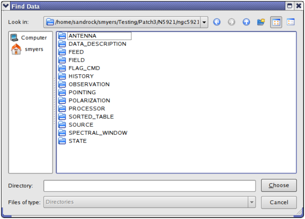
Figure 1: The contents of a MeasurementSet. These tables compose a MeasurementSet named ngc5921.demo.ms on disk. This display is obtained by using the File\:Open menu in browsetable and left double-clicking on the ngc5921.demo.ms directory.
Each “row” in a table contains entries for a number of specified “columns”. For example, in the MAIN table of the MS, the original visibility data is contained in the DATA column — each “cell” contains a matrix of observed complex visibilities for that row at a single time stamp, for a single baseline in a single spectral window. The shape of the data matrix is given by the number of channels and the number of correlations (voltage-products) formed by the correlator for an array.
Table 1 lists the non-data columns of the MAIN table that are most important during a typical data reduction session. Table 2 at the bottom lists the key data columns of the MAIN table of an interferometer MS. The MS produced by fillers for specific instruments may insert special columns, such as ALMA_PHASE_CORR, ALMA_NO_PHAS_CORR and ALMA_PHAS_CORR_FLAG_ROW for ALMA data filled using the importasdm filler. These columns are visible in browsetable and are accessible from the toolkit in the ms tool (e.g. the ms.getdata method) and from the tb “table” tool (e.g. using tb.getcol).
NOTE: When you examine table entries for IDs such as FIELD_ID or DATA_DESC_ID, you will see 0-based numbers.
Parameter |
Contents |
|---|---|
ANTENNA1 |
First antenna in baseline |
ANTENNA2 |
Second antenna in baseline |
FIELD_ID |
Field (source no.) identification |
DATA_DESC_ID |
Spectral window number, polarization identifier pair (IF no.) |
ARRAY_ID |
Subarray number |
OBSERVATION_ID |
Observation identification |
POLARIZATION_ID |
Polarization identification |
SCAN_NUMBER |
Scan number |
TIME |
Integration midpoint time |
UVW |
UVW coordinates |
Table 1: Common columns in the MAIN table of the MS.
The MS can contain a number of “scratch” columns, which are used to hold useful versions of other columns such as the data or weights for further processing. The most common scratch columns are:
CORRECTED_DATA — used to hold calibrated data for imaging or display;
MODEL_DATA — holds the Fourier inversion of a particular model image for calibration or imaging. This column is optional.
The creation and use of the scratch columns is generally done behind the scenes, but you should be aware that they are there (and when they are used).
Column |
Format |
Contents |
|---|---|---|
DATA |
Complex(Nc, Nf) |
complex visibility data matrix (= ALMA_PHASE_CORR by default) |
FLAG |
Bool(Nc, Nf) |
cumulative data flags |
WEIGHT |
Float(Nc) |
weight for a row |
SIGMA |
Float(Nc) |
sigma for a row |
WEIGHT_SPECTRUM |
Float(Nc, Nf) |
individual weights for a data matrix |
SIGMA_SPECTRUM |
Float(Nc, Nf) |
individual sigmas for a data matrix |
ALMA_PHASE_CORR |
Complex(Nc, Nf) |
on-line phase corrected data (Not in VLA data) |
ALMA_NO_PHAS_CORR |
Bool(Nc, Nf) |
data that has not been phase corrected (Not in VLA data) |
ALMA_PHAS_CORR_FLAG_RO W |
Bool(Nc, Nf) |
flag to use phase-corrected data or not (not in VLA data) |
MODEL_DATA |
Complex(Nc, Nf) |
Scratch: created by calibrater or imager tools |
CORRECTED_DATA |
Complex(Nc, Nf) |
Scratch: created by calibrater or imager tools |
Table 2: Commonly accessed MAIN Table data-related columns. NOTE: The columns ALMA_PHASE_CORR, ALMA_NO_PHAS_CORR and ALMA_PHAS_CORR_FLAG_ROW are specific to ALMA data filled using the importasdm filler.
Data flags can be set in the MS, too. Whenever a flag is set, the data will be ignored in all processing steps but not physically deleted from the MS. The flags are channel-based and stored in the MS FLAG subtable. Backups can be stored in the MS.flagversions file that can be accessed via the flagmanager.
The most recent specification for the MS is MeasurementSet definition version 2.0.
MeasurementSet v2
The MeasurementSet version 2 [3], is a database designed to hold radioastronomical data to be calibrated following the MeasurementEquation approach by Hamaker, Bregman, and Sault (1996).
Since its publication, the MeasurementSet (MS) design has been implemented by several software development groups, among them the CASA team and, e.g., the European VLBI Network team. CASA has also adopted the MeasurementEquation as its fundamental calibration scheme and has thus embraced the MS as its native way to store radio observations. With CASA becoming the designated analysis package for ALMA and the VLA, this means that the MS is now the default way of storing ALMA and VLA data during the actual analysis.
The ALMA and VLA raw data format, however, is not the MS but the so-called Astronomy Science Data Model (ASDM), also referred to as the ALMA Science Data Model for ALMA, and the Science Data Model (SDM) for the VLA. The ALMA and VLA archives hence do not store data in MS format but in ASDM format, and when a CASA user starts to work with this data, the first step has to be the import of the ASDM into the CASA MS format.
The MS is effectively a relational database which on the one hand tries to permit the storage of all imaginable radio (interferometric, single-dish) data with corresponding metadata, and on the other hand ventures to be storage-space and data-maintenance efficient by avoiding data redundancy.
The universality is achieved by offering many optional parts in the format which cover most imaginable use cases in radio astronomy. So a simple, few-antenna interferometer observing a simple object with time-independent position at just a single frequency can store its data using a small sub-set of the format while a large interferometer with antennas on time-dependent locations, observing many objects in rapid succession with time-dependent source positions using a complex, time-dependent spectral setup etc., can equally use the MS to store its data albeit using a larger subset of the possibilities of the MS.
The non-redundance of the format is achieved by simply following the standard approach of relational databases which is to put repeating pieces of information into separate database tables, the Subtables, and replacing them in the main body of the data base, the Main table, by references to the Subtables. In the case of the MS this happens in two layers of Subtables with the first layer being referenced by the Main table and the second layer being referenced by the first layer. I.e., there are some Subtables which reference other Subtables.
The Subtable referencing mechanism is defined in the original design. It works either via the line numbers of the individual Subtable ,this implies that the reference is a zero-based integer and that the removal of a line in such a Subtable requires reindexing in the referencing table(s), or via explicit references to an index column in the Subtable ,the latter is much less common.
These design principles lead to a format which puts the bulk of the data ,the interferometric visibilities and/or the single-dish total-power measurements with their timestamps, into a Main Table , and most of the metadata in the two layers of Subtables.
In the CASA MS implementation, the individual Tables are all stored in the CASA Table format, i.e. they are actually not single files on disk but directories containing several files, essentially one for each column of the table. So the entire MS is also not a single file (like, e.g., in the FITS IDI format) but a whole directory tree. For transport, the MS typically has to be turned into a single file by using the command “tar”.
The Main Table contains the radio data initially in a column called DATA (interferometric data) or FLOAT_DATA (pure single-dish data). One of these two columns always has to be present.
When a calibration is applied to the DATA column, a CORRECTED_DATA column is created to contain the calibrated data leaving the original data untouched. Furthermore, a MODEL_DATA column can be required to store expectation values for the emission of calibration sources.
For large datasets these bulk data columns can require large amounts of disk space and access to them may be slow. To mitigate these problems, the CASA team is working on making the columns “virtual” as much as possible, i.e. replacing the CORRECTED_DATA and MODEL_DATA columns by parameterised versions calculated on-the-fly.
In the case of the virtual MODEL_DATA column, this is essentially a model image which is stored with the MS and converted on-the-fly to visibilities.
In the case of the virtual CORRECTED_DATA column, this is a so-called “Cal Library” which permits to calibrate the data in the DATA column on-the-fly and make the results available as if they were stored in a standard table column.
Finally, a major case of data redundance for ALMA and VLA data is of course the fact that the raw data arrive at the user in ASDM format but then have to be translated into MS format which creates a completely redundant copy of all raw data without any gain for the user. This problem was addressed by introducing the so-called “lazy” import of ASDM data. The development is not yet completely finished but is already available for ALMA interferometric data. The idea here is to also make the DATA column virtual and perform the translation from the ASDM format on-the-fly. This typically shrinks the MS by a factor 30 in data volume. Of course the ASDM raw data has to be kept on disk for access. Access speeds to a virtual DATA column are essentially the same as to a non-virtual one. They may even be a little faster since the ASDM data is better compressed.
MS v2.0 Layout
CASA uses the MeasurementSet Version 2 (A.J. Kemball and M.H. Wieringa, eds., 2000) as the internal working data format. The MeasurementSet set was orignially defined in AIPS++ Note 191 (Wieringa and Cornwell 1996). Reproduced below is the table structrue for the MeasurementSet as used by CASA.
There is a MAIN table containing a number of data columns and keys into various subtables. There is at most one of each subtable. The subtables are stored as keywords of the MS, and all defined sub-tables are tabulated below. Optional sub-tables are shown in italics and in parentheses.
Subtables
Table |
Contents |
Keys |
|---|---|---|
ANTENNA |
Antenna characteristics |
ANTENNA_ID |
DATA_DESCRIPTION |
Data description |
DATA_DESC_ID |
(DOPPLER) |
Doppler tracking |
DOPPLER_ID, SOURCE_ID |
FEED |
Feed characteristics |
FEED_ID, ANTENNA_ID, TIME, SPECTRAL_WINDOW_ID |
FIELD |
Field position |
FIELD_ID |
FLAG_CMD |
Flag commands |
TIME |
(FREQ_OFFSET) |
Frequency offset information |
FEED_ID, ANTENNAn, FEED_ID, TIME, SPECTRAL_WINDOW_ID |
HISTORY |
History information |
OBSERVATION_ID, TIME |
OBSERVATION |
Observer, Schedule, etc |
OBSERVATION_ID |
POINTING |
Pointing information |
ANTENNA_ID, TIME |
POLARIZATION |
Polarization setup |
POLARIZATION_ID |
PROCESSOR |
Processor information |
PROCESSOR_ID |
(SOURCE) |
Source information |
SOURCE_ID, SPECTRAL_WINDOW_ID, TIME |
SPECTRAL_WINDOW |
Spectral window setups |
SPECTRAL_WINDOW_ID |
STATE |
State information |
STATE_ID |
(SYSCAL) |
System calibration characteristics |
FEED_ID, ANTENNA_ID, TIME, SPECTRAL_WINDOW_ID |
(WEATHER) |
Weather info for each antenna |
ANTENNA_ID, TIME |
Note that there are two types of subtables. For the first, simpler type, the key (ID) is the row number in the subtable. Examples are FIELD, SPECTRAL_WINDOW, OBSERVATION and PROCESSOR. For the second, the key is a collection of parameters, usually including TIME. Examples are FEED, (SOURCE), (SYSCAL), and (WEATHER).
Note that all optional columns are indicated in italics and in parentheses.
MAIN table: Data, Coordinates and Flags
Name |
Format |
Units |
Measure |
Comments |
|---|---|---|---|---|
Columns |
||||
Keywords |
||||
MS_VERSION |
Float |
MS format version |
||
(SORT_COLUMNS) |
String |
Sort columns |
||
(SORT_ORDER) |
String |
Sort order |
||
Key |
||||
TIME |
Double |
s |
EPOCH |
Integration midpoint |
(TIME_EXTRA_PREC) |
Double |
s |
extra TIME precision |
|
ANTENNA1 |
Int |
First antenna |
||
ANTENNA2 |
Int |
Second antenna |
||
(ANTENNA3) |
Int |
Third antenna |
||
FEED1 |
Int |
Feed on ANTENNA1 |
||
FEED2 |
Int |
Feed on ANTENNA2 |
||
(FEED3) |
Int |
Feed on ANTENNA3 |
||
DATA_DESC_ID |
Int |
Data desc. id. |
||
PROCESSOR_ID |
Int |
Processor id. |
||
(PHASE_ID) |
Int |
Phase id. |
||
FIELD_ID |
Int |
Field id. |
||
Non-key attributes |
||||
INTERVAL |
Double |
s |
Sampling interval |
|
EXPOSURE |
Double |
s |
The effective integration time |
|
TIME_CENTROID |
Double |
s |
EPOCH |
Time centroid |
(PULSAR_BIN) |
Int |
Pulsar bin number |
||
(PULSAR_GATE_ID) |
Int |
Pulsar gate id. |
||
SCAN_NUMBER |
Int |
Scan number |
||
ARRAY_ID |
Int |
Subarray number |
||
OBSERVATION_ID |
Int |
Observation id. |
||
STATE_ID |
Int |
State id. |
||
(BASELINE_REF) |
Bool |
Reference antenna |
||
UVW |
Double(3) |
m |
UVW |
UVW coordinates |
(UVW2) |
Double(3) |
m |
UVW |
UVW (baseline 2) |
Data |
||||
(DATA) |
Complex(Nc, Nf) |
Complex visibility matrix (synthesis arrays) |
||
(FLOAT_DATA) |
Float(Nc, Nf) |
Float data matrix (single dish) |
||
(VIDEO_POINT) |
Complex(Nc) |
Video point |
||
(LAG_DATA) |
Complex(Nc, Nl) |
Correlation function |
||
SIGMA |
Float(Nc) |
Estimated rms noise for single channel |
||
(SIGMA_SPECTRUM) |
Float(Nc, Nf*) |
Estimated rms noise |
||
WEIGHT |
Float(Nc) |
Weight for whole data matrix |
||
(WEIGHT_SPECTRUM) |
Float(Nc, Nf*) |
Weight for each channel |
||
Flag information |
||||
FLAG |
Bool(Nc, Nf*) |
Cumulative data flags |
||
FLAG_CATEGORY |
Bool(Nc, Nf*, Ncat) |
Flag categories |
||
FLAG_ROW |
Bool |
The row flag |
MS_VERSION - The MeasurementSet format revision number, expressed as \({major}_{revision}\) \({minor}_{revision}\). This version is 2.0.
SORT_COLUMNS - Sort indices, in the form \({index}_1\) \({index}_2\) \(\cdots\), for the underlying MS. A string containing “NONE” reflects no sort order. An example might be SORT_COLUMNS=”TIME ANTENNA1 ANTENNA2”, to indicate sorting in in time-baseline order.
SORT_ORDER - Sort order as either “ASCENDING” or “DESCENDING”.
TIME - Mid-point (not centroid) of data interval. Time is provided in Modified Julian Date. The CASA/casacore reference epoch (0 time) for timestamps in MeasurementSets is the MJD epoch: 1858/11/17.
TIME_EXTRA_PREC - Extra time precision.
ANTENNA n* - Antenna number (≥ 0), and a direct index into the ANTENNA sub-table rownr. For n > 2, triple-product data are implied.
FEED n* - Feed number ≥0). For n> 2, triple-product data are implied.
DATA_DESC_ID - Data description identifier (≥0), and a direct index into the DATA_DESCRIPTION sub-table rownr.
PROCESSOR_ID - Processor indentifier (≥0), and a direct index into the PROCESSOR sub-table rownr.
PHASE_ID - Switching phase identifier (≥0)
FIELD_ID - Field identifier (≥0).
INTERVAL - Data sampling interval. This is the nominal data interval and does not include the effects of bad data or partial integration.
EXPOSURE - Effective data interval, including bad data and partial averaging.
PULSAR_BIN - Pulsar bin number for the data record. Pulsar data may be measured for a limited number of pulse phase bins. The pulse phase bins are described in the PULSAR sub-table and indexed by this bin number.
PULSAR_GATE_ID - Pulsar gate identifier (≥0), and a direct index into the PULSAR_GATE sub-table rownr.
SCAN_NUMBER - Arbitrary scan number to identify data taken in the same logical scan. Not required to be unique.
ARRAY_ID - Subarray identifier (≥0), which identifies data in separate subarrays.
OBSERVATION_ID - Observation identifier (≥0), which identifies data from separate observations.
STATE_ID - State identifier (≥0), which identifies information relating to active reference signals or loads. BASELINE_REF - Flag to indicate the original correlator reference antenna for baseline-based correlators (True for ANTENNA1; False for ANTENNA2).
UVW - uvw coordinates for the baseline from ANTENNE2 to ANTENNA1, i.e. the baseline is equal to the difference POSITION2 - POSITION1. The UVW given are for the TIME_CENTROID, and correspond in general to the reference type for the PHASE_DIR of the relevant field. I.e. J2000 if the phase reference direction is given in J2000 coordinates. However, any known reference is valid. Note that the choice of baseline direction and UVW definition (W towards source direction; V in plane through source and system’s pole; U in direction of increasing longitude coordinate) also determines the sign of the phase of the recorded data.
UVW2 - uvw coordinates for the baseline from ANTENNE3 to ANTENNA1 (triple-product data only), i.e. the baseline is equal to the difference POSITION3 - POSITION1. The UVW given are for the TIME_CENTROID, and correspond in general to the reference type for the PHASE_DIR of the relevant field. I.e. J2000 if the phase reference direction is given in J2000 coordinates. However, any known reference is valid. Note that the choice of baseline direction and UVW definition (W towards source direction; V in plane through source and system’s pole; U in direction of increasing longitude coordinate) also determines the sign of the phase of the recorded data.
DATA, FLOAT_DATA, LAG_DATA - At least one of these columns should be present in a given MeasurementSet. In special cases one or more could be present (e.g., single dish data used in synthesis imaging or a mix of auto and crosscorrelations on a multi-feed single dish). If only correlation functions are stored in the MS, then Nf* is the maximum number of lags (Nl) specified in the LAG table for this LAG_ID. If both correlation functions and frequency spectra are stored in the same MS, then Nf* is the number of frequency channels, and the weight information refers to the frequency spectra only. The units for these columns (eg. ‘Jy’) specify whether the data are in flux density units or correlation coefficients.
VIDEO_POINT - The video point for the spectrum, to allow the full reverse transform.
SIGMA - The estimated rms noise for a single channel, for each correlator.
SIGMA_SPECTRUM - The estimated rms noise for each channel.
WEIGHT - The weight for the whole data matrix for each correlator, as assigned by the correlator or processor.
WEIGHT_SPECTRUM - The weight for each channel in the data matrix, as assigned by the correlator or processor. The weight spectrum should be used in preference to the WEIGHT, when available.
FLAG - An array of Boolean values with the same shape as DATA (see the DATA item above) representing the cumulative flags applying to this data matrix, as specified in FLAG_CATEGORY. Data are flagged bad if the FLAG array element is True.
FLAG_CATEGORY - An array of flag matrices with the same shape as DATA, but indexed by category. The category identifiers are specified by a keyword CATEGORY, containing an array of string identifiers, attached to the FLAG_CATEGORY column and thus shared by all rows in the MeasurementSet. The cumulative effect of these flags is reflected in column FLAG. Data are flagged bad if the FLAG array element is True. See Section 3.1.8 for further details.
FLAG_ROW - True if the entire row is flagged.
ANTENNA: Antenna Characteristics
Name |
Format |
Units |
Measure |
Comments |
|---|---|---|---|---|
Columns |
||||
Data |
||||
NAME |
String |
Antenna name |
||
STATION |
String |
Station name |
||
TYPE |
String |
Antenna type |
||
MOUNT |
String |
Mount type:alt-az, equatorial, X-Y, orbiting, bizarre |
||
POSITION |
Double(3) |
m |
POSITION |
Antenna X,Y,Z phase reference positions |
OFFSET |
Double(3) |
m |
POSITION |
Axes offset of mount to FEED REFERENCE point |
DISH_DIAMETER |
Double |
m |
Diameter of dish |
|
(ORBIT_ID) |
Int |
Orbit id. |
||
(MEAN_ORBIT) |
Double(6) |
Mean Keplerian elements |
||
(PHASED_ARRAY_ID) |
Int |
Phased array id. |
||
Flag information |
||||
FLAG_ROW |
Bool |
Row flag |
NAME - Antenna name (e.g. “NRAO_140”)
STATION - Station name (e.g. “GREENBANK”)
TYPE - Antenna type. Reserved keywords include: (“GROUND-BASED” - conventional antennas; “SPACE-BASED” - orbiting antennas; “TRACKING-STN” - tracking stations).
MOUNT - Mount type of the antenna. Reserved keywords include: (“EQUATORIAL” - equatorial mount; “ALT-AZ” - azimuth-elevation mount; “X-Y” - x-y mount; “SPACE-HALCA” - specific orientation model.)
POSITION - In a right-handed frame, X towards the intersection of the equator and the Greenwich meridian, Z towards the pole. The exact frame should be specified in the MEASURE_REFERENCE keyword (ITRF or WGS84). The reference point is the point on the az or ha axis closest to the el or dec axis.
OFFSET - Axes offset of mount to feed reference point.
DISH_DIAMETER - Nominal diameter of dish, as opposed to the effective diameter.
ORBIT_ID - Orbit identifier. Index used in ORBIT sub-table if ANTENNA_TYPE is “SPACE_BASED”.
MEAN_ORBIT - Mean Keplerian orbital elements, using the standard convention (Flatters 1998):
0: Semi-major axis of orbit (a) in m.
1: Ellipticity of orbit (e).
2: Inclination of orbit to the celestial equator (i) in deg.
3: Right ascension of the ascending node (Ω) in deg.
4: Argument of perigee (ω ) in deg.
5: Mean anomaly (M) in deg.
PHASED_ARRAY_ID - Phased array identifier. Points to a PHASED_ARRAY sub-table which points back to multiple entries in the ANTENNA sub-table and contains information on how they are combined.
FLAG_ROW - Boolean flag to indicate the validity of this entry. Set to True for an invalid row. This does not imply any flagging of the data in MAIN, but is necessary as the ANTENNA index in MAIN points directly into the ANTENNA sub-table. Thus FLAG_ROW can be used to delete an antenna entry without re-ordering the ANTENNA indices throughout the MS.
DATA_DESCRIPTION: Data Description Table
Name |
Format |
Units |
Measure |
Comments |
|---|---|---|---|---|
Columns |
||||
Data |
||||
SPECTRAL_WINDOW_ID |
Int |
Spectral window id. |
||
POLARIZATION_ID |
Int |
Polarization id. |
||
(LAG_ID) |
Int |
Lag fn. id. |
||
Flags |
||||
FLAG_ROW |
Bool |
Row flag. |
SPECTRAL_WINDOW_ID - Spectral window identifier.
POLARIZATION_ID - Polarization identifier (≥0); direct index into the POLARIZATION sub-table.
LAG_ID - Lag function identifier (≥0), and a direct index into the LAG sub-table rownr.
FLAG_ROW - True if the row does not contain valid data; does not imply flagging in MAIN.
DOPPLER: Doppler Tracking Information
Name |
Format |
Units |
Measure |
Comments |
|---|---|---|---|---|
Columns |
||||
Key |
||||
DOPPLER_ID |
Int |
Doppler tracking id. |
||
SOURCE_ID |
Int |
Source id. |
||
Data |
||||
TRANSITION_ID |
Int |
Transition id. |
||
VELDEF |
Double |
m/s |
Doppler |
Velocity definition of Doppler shift. |
DOPPLER_ID - Doppler identifier, as used in the SPECTRAL_WINDOW sub-table.
SOURCE_ID - Source identifier (as used in the SOURCE sub-table).
TRANSITION_ID - This index selects the appropriate line from the list of transitions stored for each SOURCE_ID in the SOURCE table.
VELDEF - Velocity definition of the Doppler shift, e.g., RADIO or OPTICAL velocity in m/s.
FEED: Feed Characteristics
Name |
Format |
Units |
Measure |
Comments |
|---|---|---|---|---|
Columns |
||||
Key |
||||
ANTENNA_ID |
Int |
Antenna id |
||
FEED_ID |
Int |
Feed id |
||
SPECTRAL_WINDOW_ID |
Int |
Spectral window id. |
||
TIME |
Double |
s |
EPOCH |
Interval midpoint |
INTERVAL |
Double |
s |
Time interval |
|
Data description |
||||
NUM_RECEPTORS |
Int |
receptors on this feed |
||
Data |
||||
BEAM_ID |
Int |
Beam model |
||
BEAM_OFFSET |
Double(2, NUM_RECEPTORS) |
rad |
DIRECTION |
Beam position offset (on sky but in antenna reference frame). |
(FOCUS_LENGTH) |
Double |
m |
Focus length |
|
(PHASED_FEED_ID) |
Int |
Phased feed |
||
POLARIZATION_TYPE |
String (NUM_RECEPTORS) |
Type of polarization to which a given RECEPTOR responds. |
||
POL_RESPONSE |
Complex (NUM_RECEPTORS, NUM_RECEPTORS) |
Feed polzn. response |
||
POSITION |
Double(3) |
m |
POSITION |
Position of feed relative to feed reference position for this antenna |
RECEPTOR_ANGLE |
Double (NUM_RECEPTORS) |
rad |
The reference angle for polarization. |
Notes: A feed is a collecting element on an antenna, such as a single horn, that shares joint physical properties and makes sense to calibrate as a single entity. It is an abstraction of a generic antenna feed and is considered to have one or more RECEPTORs that respond to different polarization states. A FEED may have a time-variable beam and polarization response. Feeds are numbered from 0 on each separate antenna for each SPECTRAL_WINDOW_ID. Consequently, FEED_ID should be non-zero only in the case of feed arrays, i.e. multiple, simultaneous beams on the sky at the same frequency and polarization.
ANTENNA_ID - Antenna number, as indexed from ANTENNAn in MAIN.
FEED_ID - Feed identifier, as indexed from FEEDn in MAIN.
SPECTRAL_WINDOW_ID - Spectral window identifier. A value of -1 indicates the row is valid for all spectral windows.
TIME - Mid-point of time interval for which the feed parameters in this row are valid. The same Measure reference used for the TIME column in MAIN must be used.
INTERVAL - Time interval.
NUM_RECEPTORS - Number of receptors on this feed. See POLARIZATION_TYPE for further information.
BEAM_ID - Beam identifier. Points to an optional BEAM sub-table defining the primary beam and polarization response for this FEED. A value of -1 indicates that no associated beam response is defined.
BEAM_OFFSET - Beam position offset, as defined on the sky but in the antenna reference frame.
FOCUS_LENGTH - Focus length. As defined along the optical axis of the antenna.
PHASED_FEED_ID - Phased feed identifier. Points to a PHASED_FEED sub-table which in turn points back to multiple entries in the FEED table, and specifies the manner in which they are combined.
POLARIZATION_TYPE - Polarization type to which each receptor responds (e.g. “R”,”L”,”X” or “Y”). This is the receptor polarization type as recorded in the final correlated data (e.g. “RR”); i.e. as measured after all polarization combiners.
POL_RESPONSE - Polarization response at the center of the beam for this feed. Expressed in a linearly polarized basis ($ \textbf{\vec e_x}`$, $ :nbsphinx-math:textbf{vec e_y}`$) using the IEEE convention.
POSITION - Offset of feed relative to the feed reference position for this antenna (see ANTENNA sub-table).
RECEPTOR_ANGLE - Polarization reference angle. Converts into parallactic angle in the sky domain.
FIELD: Field Positions for Each Source
Name |
Format |
Units |
Measure |
Comments |
|---|---|---|---|---|
Columns |
||||
Key |
||||
Data |
||||
NAME |
String |
Name of field |
||
CODE |
String |
Special characteristics of field |
||
TIME |
Double |
s |
EPOCH |
Time origin for the directions and rates |
NUM_POLY |
Int |
Series order |
||
DELAY_DIR |
Double(2, NUM_POLY+1) |
rad |
DIRECTION |
Direction of delay center. |
PHASE_DIR |
Double(2, NUM_POLY+1) |
rad |
DIRECTION |
Phase center. |
REFERENCE_DIR |
Double(2, NUM_POLY+1) |
rad |
DIRECTION |
Reference center |
SOURCE_ID |
Int |
Index in Source table |
||
(EPHEMERIS_ID) |
Int |
Ephemeris id. |
||
Flags |
||||
FLAG_ROW |
Bool |
Row flag |
NAME - Field name; user specified.
CODE - Field code indicating special characteristics of the field; user specified.
TIME - Time reference for the directions and rates. Required to use the same TIME Measure reference as in MAIN.
NUM_POLY - Series order for the *_DIR columns.
DELAY_DIR - Direction of delay center; can be expressed as a polynomial in time. Final result converted to the defined Direction Measure type.
PHASE_DIR - Direction of phase center; can be expressed as a polynomial in time. Final result converted to the defined Direction Measure type.
REFERENCE_DIR - Reference center; can be expressed as a polynomial in time. Final result converted to the defined Direction Measure type. Used in single-dish to record the associated reference direction if position-switching has already been applied. For interferometric data, this is the original correlated field center, and may equal DELAY_DIR or PHASE_DIR.
SOURCE_ID - Points to an entry in the optional SOURCE subtable, a value of -1 indicates there is no corresponding source defined.
EPHEMERIS_ID - Points to an entry in the EPHEMERIS sub-table, which defines the ephemeris used to compute the field position. Useful for moving, near-field objects, where the ephemeris may be revised over time.
FLAG_ROW - True if data in this row are invalid, else False. Does not imply flagging in MAIN.
FLAG_CMD: Flag Commands
Name |
Format |
Units |
Measure |
Comments |
|---|---|---|---|---|
Columns |
||||
Key |
||||
TIME |
Double |
s |
EPOCH |
Mid-point of interval |
INTERVAL |
Double |
s |
Time interval |
|
Data |
||||
TYPE |
String |
FLAG or UNFLAG |
||
REASON |
String |
Flag reason |
||
LEVEL |
Int |
Flag level |
||
SEVERITY |
Int |
Severity code |
||
APPLIED |
Bool |
True if applied in MAIN |
||
COMMAND |
String |
Flag command |
TIME - Mid-point of the time interval to which this flagging command applies. Required to use the same TIME Measure reference as used in MAIN.
INTERVAL - Time interval.
TYPE - Type of flag command, representing either a flagging (“FLAG”) or un-flagging (“UNFLAG”) operation.
REASON - Flag reason; user specified.
LEVEL - Flag level (≥0); reflects different revisions of flags which have the same REASON.
SEVERITY - Severity code for the flag, on a scale of 0-10 in order of increasing severity; user specified.
APPLIED - True if this flag has been applied to MAIN, and update in FLAG_CATEGORY and FLAG. False if this flag has not been applied to MAIN.
COMMAND - Global flag command, expressed in the standard syntax for data selection, as adopted within the project as a whole.
FREQ_OFFSET: Frequency Offset Information
Name |
Format |
Units |
Measure |
Comments |
|---|---|---|---|---|
Columns |
||||
Key |
||||
ANTENNA1 |
Int |
Antenna 1. |
||
ANTENNA2 |
Int |
Antenna 2. |
||
FEED_ID |
Int |
Feed id. |
||
SPECTRAL_WINDOW_ID |
Int |
Spectral window id. |
||
TIME |
Double |
s |
EPOCH |
Interval midpoint |
INTERVAL |
Double |
s |
Time interval |
|
Data |
||||
OFFSET |
Double |
Hz |
Frequency offset |
ANTENNA n* - Antenna identifier, as indexed from ANTENNAn in MAIN.
FEED_ID - Antenna identifier, as indexed from FEEDn in MAIN.
SPECTRAL_WINDOW_ID - Spectral window identifier.
TIME - Mid-point of the time interval for which this offset is valid. Required to use the same TIME Measure reference as used in MAIN.
INTERVAL - Time interval.
OFFSET - Frequency offset to be added to the frequency axis for this spectral window, as defined in the SPECTRAL_WINDOW sub-table. Required to have the same Frequency Measure reference as CHAN_FREQ in that table.
HISTORY: History Information
Name |
Format |
Units |
Measure |
Comments |
|---|---|---|---|---|
Columns |
||||
Key |
||||
TIME |
Double |
s |
EPOCH |
Time-stamp for message |
OBSERVATION_ID |
Int |
Points to OBSERVATION table |
||
Data |
||||
MESSAGE |
String |
Log message |
||
PRIORITY |
String |
Message priority |
||
ORIGIN |
String |
Code origin |
||
OBJECT_ID |
String |
Originating ObjectID |
||
APPLICATION |
String |
Application name |
||
CLI_COMMAND |
String(*) |
CLI command sequence |
||
APP_PARAMS |
String(*) |
Application paramters |
TIME - Time-stamp for the history record. Required to have the same TIME Measure reference as used in MAIN.
OBSERVATION_ID - Observation identifier (see the OBSERVATION table)
MESSAGE - Log message.
PRIORITY - Message priority, with allowed types: (“DEBUGGING”, “WARN”, “NORMAL”, or “SEVERE”).
ORIGIN - Source code origin from which message originated.
OBJECT_ID - Originating ObjectID, if available, else blank.
APPLICATION - Application name.
CLI_COMMAND - CLI command sequence invoking the application.
APP_PARAMS - Application parameter values, in the adopted project-wide format.
OBSERVATION: Observation Information
Name |
Format |
Units |
Measure |
Comments |
|---|---|---|---|---|
Columns |
||||
Data |
||||
TELESCOPE_NAME |
String |
Telescope name |
||
TIME_RANGE |
Double(2) |
s |
EPOCH |
Start, end times |
OBSERVER |
String |
Name of observer(s) |
||
LOG |
String(*) |
Observing log |
||
SCHEDULE_TYPE |
String |
Schedule type |
||
SCHEDULE |
String(*) |
Project schedule |
||
PROJECT |
String |
Project identification string. |
||
RELEASE_DATE |
Double |
s |
EPOCH |
Target release date |
Flags |
||||
FLAG_ROW |
Bool |
Row flag. |
TELESCOPE_NAME - Telescope name (e.g. “WSRT” or “VLBA”).
TIME_RANGE - The start and end times of the overall observing period spanned by the actual recorded data in MAIN. Required to use the same TIME Measure reference as in MAIN. Time is provided in Modified Julian Date. The CASA/casacore reference epoch (0 time) for timestamps in MeasurementSets is the MJD epoch: 1858/11/17.
OBSERVER - The name(s) of the observer(s).
LOG - The observing log, as supplied by the telescope or instrument.
SCHEDULE_TYPE - The schedule type, with current reserved types (“VLBA-CRD”, “VEX”, “WSRT”, “ATNF”).
SCHEDULE - Unmodified schedule file, of the type specified, and as used by the instrument.
PROJECT - Project code (e.g. “BD46”)
RELEASE_DATE - Project release date. This is the date on which the data may become public.
FLAG_ROW - Row flag. True if data in this row is invalid, but does not imply any flagging in MAIN.
POINTING: Antenna Pointing Information
Name |
Format |
Units |
Measure |
Comments |
|---|---|---|---|---|
Columns |
||||
Key |
||||
ANTENNA_ID |
Int |
Antenna id. |
||
TIME |
Double |
s |
EPOCH |
Interval midpoint |
INTERVAL |
Double |
s |
Time interval |
|
Data |
||||
NAME |
String |
Pointing position desc. |
||
NUM_POLY |
Int |
Series order |
||
TIME_ORIGIN |
Double |
s |
EPOCH |
Origin for the polynomial |
DIRECTION |
Double(2, NUM_POLY+1) |
rad |
DIRECTION |
Antenna pointing direction |
TARGET |
Double(2, NUM_POLY+1) |
rad |
DIRECTION |
Target direction |
(POINTING_OFFSET) |
Double(2, NUM_POLY+1) |
rad |
DIRECTION |
A priori pointing correction |
(SOURCE_OFFSET) |
Double(2, NUM_POLY+1) |
rad |
DIRECTION |
Offset from source |
(ENCODER) |
Double(2) |
rad |
DIRECTION |
Encoder values |
(POINTING_MODEL_ID) |
Int |
Pointing model id. |
||
TRACKING |
Bool |
True if on-position |
||
(ON_SOURCE) |
Bool |
True if on-source |
||
(OVER_THE_TOP) |
Bool |
True if over the top |
ANTENNA_ID - Antenna identifier, as specified by ANTENNAn in MAIN.
TIME - Mid-point of the time interval for which the information in this row is valid. Required to use the same TIME Measure reference as in MAIN.
INTERVAL - Time interval.
NAME - Pointing direction name; user specified.
NUM_POLY - Series order for the polynomial expressions in DIRECTION and POINTING_OFFSET.
TIME_ORIGIN - Time origin for the polynomial expansions.
DIRECTION - Antenna pointing direction, optionally expressed as polynomial coefficients. The final result is interpreted as a Direction Measure using the specified Measure reference.
TARGET - Target pointing direction, optionally expressed as polynomial coefficients. The final result is interpreted as a Direction Measure using the specified Measure reference. This is the true expected position of the source, including all coordinate corrections such as precession, nutation etc.
POINTING_OFFSET - The a priori pointing corrections applied by the telescope in pointing to the DIRECTION position, optionally expressed as polynomial coefficients. The final result is interpreted as a Direction Measure using the specified Measure reference.
SOURCE_OFFSET - The commanded offset from the source position, if offset pointing is being used.
ENCODER - The current encoder values on the primary axes of the mount type for the antenna, expressed as a Direction Measure.
TRACKING - True if tracking the nominal pointing position.
ON-SOURCE - True if the nominal pointing direction coincides with the source, i.e. offset-pointing is not being used.
OVER-THE-TOP - True if the antenna was driven to this position “over the top” (az-el mount).
POLARIZATION: Polarization Setup Information
Name |
Format |
Units |
Measure |
Comments |
|---|---|---|---|---|
Columns |
||||
Data description columns |
||||
NUM_CORR |
Int |
correlations |
||
Data |
||||
CORR_TYPE |
Int(NUM_CORR) |
Polarization of correlation |
||
CORR_PRODUCT |
Int(2, NUM_CORR) |
Receptor cross-products |
||
Flags |
||||
FLAG_ROW |
Bool |
Row flag |
NUM_CORR- The number of correlation polarization products. For example, for (RR) this value would be 1, for (RR, LL) it would be 2, and for (XX,YY,XY,YX) it would be 4, etc.
CORR_TYPE - An integer for each correlation product indicating the Stokes type as defined in the Stokes class enumeration.
CORR_PRODUCT - Pair of integers for each correlation product, specifying the receptors from which the signal originated. The receptor polarization is defined in the POLARIZATION_TYPE column in the FEED table. An example would be (0,0), (0,1), (1,0), (1,1) to specify all correlations between two receptors.
FLAG_ROW - Row flag. True is the data in this row are not valid, but does not imply the flagging of any DATA in MAIN.
PROCESSOR: Processor Information
Name |
Format |
Units |
Measure |
Comments |
|---|---|---|---|---|
Columns |
||||
Data |
||||
TYPE |
String |
Processor type |
||
SUB_TYPE |
String |
Processor sub-type |
||
TYPE_ID |
Int |
Processor type id. |
||
MODE_ID |
Int |
Processor mode id. |
||
(PASS_ID) |
Int |
Processor pass number |
||
Flags |
||||
FLAG_ROW |
Bool |
Row flag |
TYPE - Processor type; reserved keywords include (“CORRELATOR” - interferometric correlator; “SPECTROMETER” - single-dish correlator; “RADIOMETER” - generic detector/integrator; “PULSAR-TIMER” - pulsar timing device).
SUB_TYPE - Processor sub-type, e.g. “GBT” or “JIVE”.
TYPE_ID - Index used in a specialized sub-table named as subtype_type, which contains time-independent processor information applicable to the current data record (e.g. a JIVE_CORRELATOR sub-table). Time-dependent information for each device family is contained in other tables, dependent on the device type.
MODE_ID - Index used in a specialized sub-table named as subtype_type_mode, containing information on the processor mode applicable to the current data record. (e.g. a GBT_SPECTROMETER_MODE sub-table).
PASS_ID - Pass identifier; this is used to distinguish data records produced by multiple passes through the same device, where this is possible (e.g. VLBI correlators). Used as an index into the associated table containing pass information.
FLAG_ROW - Row flag. True if data in the row is not valid, but does not imply flagging in MAIN.
SOURCE: Source Information
Name |
Format |
Units |
Measure |
Comments |
|---|---|---|---|---|
Columns |
||||
Key |
||||
SOURCE_ID |
Int |
Source id |
||
TIME |
Double |
s |
EPOCH |
Midpoint of time for which this set of parameters is accurate |
INTERVAL |
Double |
s |
Interval |
|
SPECTRAL_WINDOW_ID |
Int |
Spectral Window id |
||
Data description |
||||
NUM_LINES |
Int |
Number of spectral lines |
||
Data |
||||
NAME |
String |
Name of source as given during observations |
||
CALIBRATION_GROUP |
Int |
grouping for calibration purpose |
||
CODE |
String |
Special characteristics of source, e.g. Bandpass calibrator |
||
DIRECTION |
Double(2) |
rad |
DIRECTION |
Direction (e.g. RA, DEC) |
(POSITION) |
Double(3) |
m |
POSITION |
Position (e.g. for solar system objects) |
PROPER_MOTION |
Double(2) |
rad/s |
Proper motion |
|
(TRANSITION) |
String(NUM_LINES) |
Transition name |
||
(REST_FREQUENCY) |
Double(NUM_LINES) |
Hz |
FREQUENCY |
Line rest frequency |
(SYSVEL) |
Double(NUM_LINES) |
m/s |
RADIAL VELOCITY |
Systemic velocity at reference |
(SOURCE_MODEL) |
TableRecord |
Default csm |
||
(PULSAR_ID) |
Int |
Pulsar id. |
SOURCE_ID - Source identifier (≥ 0), as specified in the FIELD sub-table.
TIME - Mid-point of the time interval for which the data in this row is valid. Required to use the same TIME Measure reference as in MAIN.
INTERVAL - Time interval.
SPECTRAL_WINDOW_ID - Spectral window identifier. A -1 indicates that the row is valid for all spectral windows.
NUM_LINES - Number of spectral line transitions associated with this source and spectral window id. combination.
NAME - Source name; user specified.
CALIBRATION_GROUP - Calibration group number to which this source belongs; user specified.
CODE - Source code, used to describe any special characteristics f the source, such as the nature of a calibrator. Reserved keyword, including (“BANDPASS CAL”).
DIRECTION - Source direction at this TIME.
POSITION - Source position (x, y, z) at this TIME (for near-field objects).
PROPER_MOTION - Source proper motion at this TIME.
TRANSITION - Transition names applicable for this spectral window (e.g. “v=1, J=1-0, SiO”).
REST_FREQUENCY - Rest frequencies for the transitions.
SYSVEL - Systemic velocity for each transition.
SOURCE_MODEL - Reference to an assigned component source model table.
PULSAR_ID - An index used in the PULSAR sub-table to define further pulsar-specific properties if the source is a pulsar.
SPECTRAL_WINDOW: Spectral Window Description
Name |
Format |
Units |
Measure |
Comments |
|---|---|---|---|---|
Columns |
||||
Data description columns |
||||
NUM_CHAN |
Int |
spectral channels |
||
Data |
||||
NAME |
String |
Spectral window name |
||
REF_FREQUENCY |
Double |
Hz |
FREQUENCY |
The reference frequency. |
CHAN_FREQ |
Double(NUM_CHAN) |
Hz |
FREQUENCY |
Center frequencies for each channel in the data matrix. |
CHAN_WIDTH |
Double(NUM_CHAN) |
Hz |
Channel width for each channel in the data matrix. |
|
MEAS_FREQ_REF |
Int |
FREQUENCY Measure ref. |
||
EFFECTIVE_BW |
Double(NUM_CHAN) |
Hz |
The effective noise bandwidth of each spectral channel |
|
RESOLUTION |
Double(NUM_CHAN) |
Hz |
The effective spectral resolution of each channel |
|
TOTAL_BANDWIDTH |
Double |
Hz |
total bandwidth for this window |
|
NET_SIDEBAND |
Int |
Net sideband |
||
(BBC_NO) |
Int |
Baseband converter no. |
||
(BBC_SIDEBAND) |
Int |
BBC sideband |
||
IF_CONV_CHAIN |
Int |
The IF conversion chain |
||
(RECEIVER_ID) |
Int |
Receiver id. |
||
FREQ_GROUP |
Int |
Frequency group |
||
FREQ_GROUP_NAME |
String |
Freq. group name |
||
(DOPPLER_ID) |
Int |
Doppler id. |
||
(ASSOC_SPW_ID) |
Int(*) |
Associated spw_id. |
||
(ASSOC_NATURE) |
String(*) |
Nature of association |
||
Flags |
||||
FLAG_ROW |
Bool |
NUM_CHAN - Number of spectral channels.
NAME - Spectral window name; user specified.
REF_FREQUENCY - The reference frequency. A frequency representative of this spectral window, usually the sky frequency corresponding to the DC edge of the baseband. Used by the calibration system if a fixed scaling frequency is required or in algorithms to identify the observing band.
CHAN_FREQ - Center frequencies for each channel in the data matrix. These can be frequency-dependent, to accommodate instruments such as acousto-optical spectrometers. Note that the channel frequencies may be in ascending or descending frequency order.
CHAN_WIDTH - Nomical channel width of each spectral channel. Although these can be derived from CHAN_FREQ by differencing, it is more efficient to keep a separate reference to this information.
MEAS_FREQ_REF - Frequency Measure reference for CHAN_FREQ. This allows a row-based reference for this column in order to optimize the choice of Measure reference when Doppler tracking is used. Modified only by the MS access code.
EFFECTIVE_BW - The effective noise bandwidth of each spectral channel.
RESOLUTION - The effective spectral resolution of each channel.
TOTAL_BANDWIDTH - The total bandwidth for this spectral window.
NET_SIDEBAND - The net sideband for this spectral window.
BBC_NO - The baseband converter number, if applicable.
BBC_SIDEBAND - The baseband converter sideband, is applicable.
IF_CONV_CHAIN - Identification of the electronic signal path for the case of multiple (simultaneous) IFs. (e.g. VLA: AC=0, BD=1, ATCA: Freq1=0, Freq2=1)
RECEIVER_ID - Index used to identify the receiver associated with the spectral window. Further state information is planned to be stored in a RECEIVER sub-table.
FREQ_GROUP - The frequency group to which the spectral window belongs. This is used to associate spectral windows for joint calibration purposes.
FREQ_GROUP_NAME - The frequency group name; user specified.
DOPPLER_ID - The Doppler identifier defining frame information for this spectral window.
ASSOC_SPW_ID - Associated spectral windows, which are related in some fashion (e.g. “channel-zero”).
ASSOC_NATURE - Nature of the association for ASSOC_SPW_ID; reserved keywords are (“CHANNEL-ZERO” - channel zero; “EQUAL-FREQUENCY” - same frequency labels; “SUBSET” - narrow-band subset).
FLAG_ROW - True if the row does not contain valid data.
STATE: State Information
Name |
Format |
Units |
Measure |
Comments |
|---|---|---|---|---|
Columns |
||||
Data |
||||
SIG |
Bool |
Signal |
||
REF |
Bool |
Reference |
||
CAL |
Double |
K |
Noise calibration |
|
LOAD |
Double |
K |
Load temperature |
|
SUB_SCAN |
Int |
Sub-scan number |
||
OBS_MODE |
String |
Observing mode |
||
Flags |
||||
FLAG_ROW |
Bool |
Row flag |
SIG - True if the source signal is being observed.
REF - True for a reference phase.
CAL - Noise calibration temperature (zero if not added).
LOAD - Load temperature (zero if no load).
SUB_SCAN - Sub-scan number (≥ 0), relative to the SCAN_NUMBER in MAIN. Used to identify observing sequences.
OBS_MODE - Observing mode; defined by a set of reserved keywords characterizing the current observing mode (e.g. “OFF-SPECTRUM”). Used to define the schedule strategy.
FLAG_ROW - True if the row does not contain valid data. Does not imply flagging in MAIN.
SYSCAL: System Calibration
Name |
Format |
Units |
Measure |
Comments |
|---|---|---|---|---|
Columns |
||||
Key |
||||
ANTENNA_ID |
Int |
Antenna id |
||
FEED_ID |
Int |
Feed id |
||
SPECTRAL_WINDOW_ID |
Int |
Spectral window id |
||
TIME |
Double |
s |
EPOCH |
Midpoint of time for which this set of parameters is accurate |
INTERVAL |
Double |
s |
Interval |
|
Data |
||||
(PHASE_DIFF) |
Float |
rad |
Phase difference between receptor 0 and receptor 1 |
|
(TCAL) |
Float (Nr) |
K |
Calibration temp |
|
(TRX) |
Float (Nr) |
K |
Receiver temperature |
|
(TSKY) |
Float (Nr) |
K |
Sky temperature |
|
(TSYS) |
Float (Nr) |
K |
System temp |
|
(TANT) |
Float (Nr) |
K |
Antenna temperature |
|
(TANT_TSYS) |
Float(Nr) |
$ {{T_{ant}}:nbsphinx-math:over{T_{sys}}}$ |
||
(TCAL_SPECTRUM) |
Float (Nr, Nf) |
K |
Calibration temp |
|
(TRX_SPECTRUM) |
Float (Nr, Nf) |
K |
Receiver temperature |
|
(TSKY_SPECTRUM) |
Float (Nr, Nf) |
K |
Sky temperature spectrum |
|
(TSYS_SPECTRUM) |
Float (Nr, Nf) |
K |
System temp |
|
(TANT_SPECTRUM) |
Float (Nr, Nf) |
K |
Antenna temperature spectrum |
|
(TANT_TSYS_SPECTRUM) |
Float (Nr,Nf) |
$ {{T_{ant}}:nbsphinx-math:over{T_{sys}}}$ spectrum |
||
Flags |
||||
(PHASE_DIFF_FLAG) |
Bool |
Flag for PHASE_DIFF |
||
(TCAL_FLAG) |
Bool |
Flag for TCAL |
||
(TRX_FLAG) |
Bool |
Flag for TRX |
||
(TSKY_FLAG) |
Bool |
Flag for TSKY |
||
(TSYS_FLAG) |
Bool |
Flag for TSYS |
||
(TANT_FLAG) |
Bool |
Flag for TANT |
||
(TANT_TSYS_FLAG) |
Bool |
Flag for \({{T_{ant}}\over{T_{sys}}}\) |
ANTENNA_ID - Antenna identifier, as indexed by ANTENNAn in MAIN.
FEED_ID - Feed identifier, as indexed by FEEDn in MAIN.
SPECTRAL_WINDOW_ID - Spectral window identifier.
TIME - Mid-point of the time interval for which the data in this row are valid. Required to use the same TIME Measure reference as that in MAIN.
INTERVAL - Time interval.
PHASE_DIFF - Phase difference between receptor 0 and receptor 1.
TCAL - Calibration temperature.
TRX - Receiver temperature.
TSKY - Sky temperature.
TSYS - System temperature.
TANT - Antenna temperature.
TANT_TSYS - Antenna temperature over system temperature.
TCAL_SPECTRUM - Calibration temperature spectrum.
TRX_SPECTRUM - Receiver temperature spectrum.
TSKY_SPECTRUM - Sky temperature spectrum.
TSYS_SPECTRUM - System temperature spectrum.
TANT_SPECTRUM - Antenna temperature spectrum.
TANT_TSYS_SPECTRUM - Antenna temperature over system temperature spectrum.
PHASE_DIFF_FLAG - True if PHASE_DIFF flagged.
TCAL_FLAG - True if TCAL flagged.
TRX_FLAG - True if TRX flagged.
TSKY_FLAG - True if TSKY flagged.
TSYS_FLAG - True if TSYS flagged.
TANT_FLAG - True if TANT flagged.
TANT_TSYS_FLAG - True if TANT_TSYS flagged.
WEATHER: Weather Station Information
Name |
Format |
Units |
Measure |
Comments |
|---|---|---|---|---|
Columns |
||||
Key |
||||
ANTENNA_ID |
Int |
Antenna number |
||
TIME |
Double |
s |
EPOCH |
Mid-point of interval |
INTERVAL |
Double |
s |
Interval over which data is relevant |
|
Data |
||||
(H2O) |
Float |
m-2 |
Average column density of water |
|
(IONOS_ELECTRON) |
Float |
m-2 |
Average column density of electrons |
|
(PRESSURE) |
Float |
hPa |
Ambient atmospheric pressure |
|
(REL_HUMIDITY) |
Float |
Ambient relative humidity |
||
(TEMPERATURE) |
Float |
K |
Ambient air temperature for an antenna |
|
(DEW_POINT) |
Float |
K |
Dew point |
|
(WIND_DIRECTION) |
Float |
rad |
Average wind direction |
|
(WIND_SPEED) |
Float |
m/s |
Average wind speed |
|
Flags |
||||
(H2O_FLAG) |
Bool |
Flag for H2O |
||
(IONOS_ELECTRON_FLAG) |
Bool |
Flag for IONOS_ELECTRON |
||
(PRESSURE_FLAG) |
Bool |
Flag for PRESSURE |
||
(REL_HUMIDITY_FLAG) |
Bool |
Flag for REL_HUMIDITY |
||
(TEMPERATURE_FLAG) |
Bool |
Flag for TEMPERATURE |
||
(DEW_POINT_FLAG) |
Bool |
Flag for DEW_POINT |
||
(WIND_DIRECTION_FLAG) |
Bool |
Flag for WIND_DIRECTION |
||
(WIND_SPEED_FLAG) |
Bool |
Flag for WIND_SPEED |
ANTENNA_ID - Antenna identifier, as indexed by ANTENNAn from MAIN.
TIME - Mid-point of the time interval over which the data in the row are valid. Required to use the same TIME Measure reference as in MAIN.
INTERVAL - Time interval.
H2O - Average column density of water.
IONOS_ELECTRON - Average column density of electrons.
PRESSURE - Ambient atmospheric pressure.
REL_HUMIDITY - Ambient relative humidity.
TEMPERATURE - Ambient air temperature.
DEW_POINT - Dew point temperature.
WIND_DIRECTION - Average wind direction.
WIND_SPEED - Average wind speed.
H2O_FLAG - Flag for H2O.
IONOS_ELECTRON_FLAG - Flag for IONOS_ELECTRON.
PRESSURE_FLAG - Flag for PRESSURE.
REL_HUMIDITY_FLAG - Flag for REL_HUMIDITY.
TEMPERATURE_FLAG - Flag for TEMPERATURE.
DEW_POINT_FLAG - Flag for DEW_POINT.
WIND_DIRECTION_FLAG - Flag for DEW_POINT.
WIND_SPEED_FLAG - Flag for DEW_POINT.
Definition Synthesized Beam
CASA uses the following zero-centered two dimensional elliptical Gaussian function or Gaussian beam:
where A is the amplitude (usually set to unity) and \(\theta\) is the anti-clockwise angle from the x axis to the line that lies along the greatest width of \(f(x,y)\) (the line and the x axis must be coplanar). The factors \(d_1\) and \(d_2\) are respectively the semi-major and semi-minor axis of the ellipse, which is formed by the cross-section that lies parallel to the \(x, y\) plane, at a height so that \(d_1\) is equal to the FWHM (full width at half maximum) distance of the one dimensional Gaussian which lies on the plane formed by the \(z\) axis and \(d_1\). Note that \(d_1 \geqslant d_2 > 0\), since \(d_1\) is the semi-major axis.
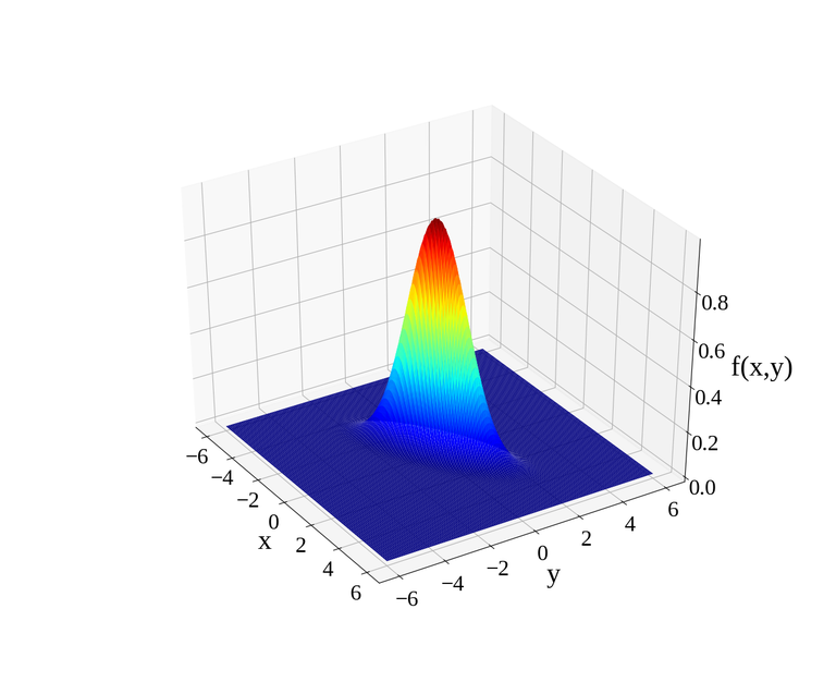
Figure 1: Surface plot of a two dimensional elliptical Gaussian with \(A = 1\), \(d_1 = 3\), \(d_2=1\) and \(\theta = 30^\circ\).
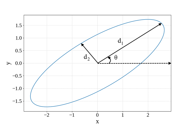
Figure 2: Cross-section parallel to the \(x, y\) plane of the two dimensional elliptical Gaussian from Fig. 1, where the resulting ellipse has a semi-major and semi-minor axis equal to \(d_1\) and \(d_2\), respectively.
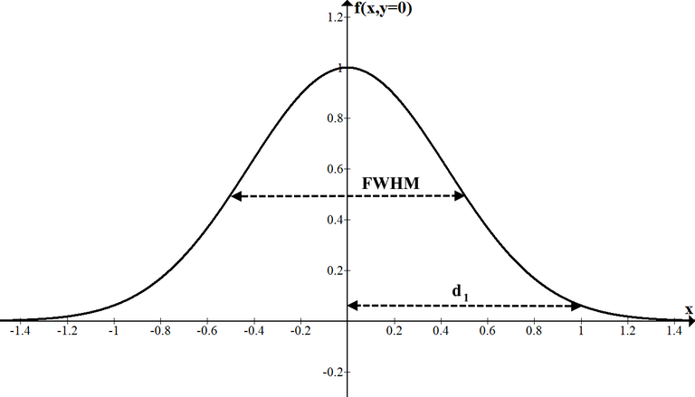
Figure 3: One dimensional Gaussian plot for \(A = 1\), \(y = 0\), \(\theta = 0\) and \(d_1 = 1 = FWHM\).
For calculating the Fourier transform of the two dimensional elliptical Gaussian, the above Equation can be re-written by grouping the \(x\) and \(y\) terms:
where
Converting from \(\alpha\), \(\beta\), \(\gamma\) to \(d_1\), \(d_2\), \(\theta\) can be done using the following set of equations:
Working with MS Data
The ALMA and VLA raw data are stored in their respective archives in the Astronomy Science Data Model (ASDM) format. The definition of the format can be found here.
To bring them into CASA, the ASDMs are filled into a so-called MeasurementSet (or MS) (format description can be found here). In its logical structure, the MS looks like a generalized description of data from any interferometric or single dish telescope. Physically, the MS consists of several tables in a directory on disk, in XML format.
Tables in CASA are actually directories containing files that are the sub-tables. For example, when you create a MS called AM675.ms, then the name of the directory where all the tables are stored will be called AM675.ms/. See chapter “Visibility Data Import Export” for more information on MeasurementSet and Data Handling in CASA.
The data that you originally get from a telescope can be put in any directory that is convenient to you. Once you “fill” the data into a MeasurementSet that can be accessed by CASA, it is generally best to keep that MS in the same directory where you started CASA so you can get access to it easily (rather than constantly having to specify a full path name).
When you generate calibration solutions or images (again these are in table format), these will also be written to disk. It is a good idea to keep them in the directory in which you started CASA, too.
How do I get rid of my data in CASA?
Note that when you delete a MeasurementSet, calibration table, or image, which are in fact directories, you must delete this and all underlying directories and files. If you are not running CASA, this is most simply done by using the file delete method of the operating system from which you started CASA. For example, when running CASA on a Linux system, in order to delete the MeasurementSet named AM675.ms type
CASA <5>: !rm -r AM675.ms
from within CASA. The ! tells CASA that a system command follows, and the -r makes sure that all subdirectories are deleted recursively.
It is convenient to prefix all MS, calibration tables, and output files produced in a run with a common string. For example, one might prefix all files from VLA project AM675 with AM675, e.g. AM675.ms, AM675.cal, AM675.clean. Then,
CASA <6>: !rm -r AM675*
will clean up all of these.
In scripts, the ! escape to the OS will not work. Instead, use the os.system() function to do the same thing:
os.system('rm -r AM675*')
If you are within CASA, then the CASA system is keeping a cache of tables that you have been using and using the OS to delete them will confuse things. For example, running a script that contains rm commands multiple times will often not run or crash the second time as the cache gets confused. The clean way of removing CASA tables (MS, caltables, images) inside CASA is to use the rmtables task:
rmtables('AM675.ms')
and this can also be wildcarded (though you may get warnings if it tries to delete files or directories that fit the name wildcard that are not CASA tables).
ALERT: rmtables is the preferred way to remove data. clean is a good example where frequently data are left in the cache after deleting the output files via “!rm -r”. Restarting clean then sometimes claims that the files still exist, even though they are not present on disk anymore. rmtables will completely remove the files on disks and all cached versions and restarting clean will work as intended.
ALERT: Some CASA processes lock the file and forget to give it up when they are done. You will get WARNING messages from rmtables and your script will probably crash second time around as the file isn’t removed. The safest thing is still to exit CASA and start a new session for multiple runs.
What’s in my data?
The actual data is in a large MAIN table that is organized in such a way that you can access different parts of the data easily. This table contains a number of “rows”, which are effectively a single timestamp for a single spectral window (like an IF from the VLA) and a single baseline (for an interferometer).
There are a number of “columns” in the MS, the most important of which for our purposes is the DATA column — this contains the original visibility data from when the MS was created or filled. There are other helpful “scratch” columns which hold useful versions of the data or weights for further processing: the CORRECTED_DATA column, which is used to hold calibrated data and an optional MODEL_DATA column, which may hold the Fourier inversion of a particular model image. The creation and use of the scratch columns is generally done behind the scenes, but you should be aware that they are there (and when they are used). We will occasionally refer to the rows and columns in the MS.
Loading Data to Images
The subsections below provide a brief overview of the steps you will need to load data into CASA and obtain a final, calibrated image. Each subject is covered in more detail in other chapters.
An end-to-end workflow diagram for CASA data reduction for interferometry data is shown in the Figure below. This might help you chart your course through the package. In the following sub-sections, we will chart a rough course through this process, with the later chapters filling in the individual boxes.
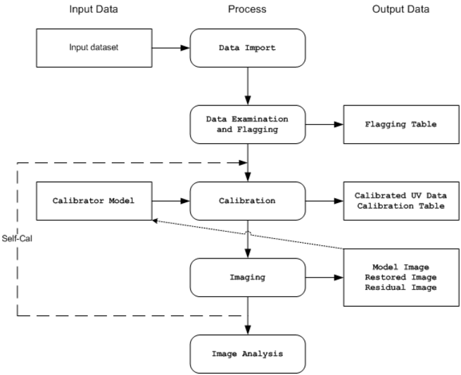
Flow chart of the data processing operations that a general user will carry out in an end-to-end CASA reduction session.
Note that single-dish data reduction (for example with the ALMA single-dish system) follows a similar course. This is detailed in the corresponding chapters.
Loading Data into CASA
The key data and image import tasks are (see “Visibility Data Import Export”):
importuvfits — import visibility data in UVFITS format
importvla — import data from VLA that is in export format
importasdm — import data in ASDM format
importfits — import a FITS image into a CASA image format table
These are used to bring in your interferometer data, to be stored as a CASA MeasurementSet (MS), and any previously made images or models (to be stored as CASA image tables).
The data import tasks will create a MS with a path and name specified by the vis parameter. The MeasurementSet is the internal data format used by CASA, and conversion from any other native format is necessary for most of the data reduction tasks.
Once data is imported, there are other operations you can use to manipulate the datasets:
concat — concatenate multiple MSs into a given or a new MS
Data Examination, Editing, and Flagging
The main data examination and flagging tasks are:
listobs — summarize the contents of a MS
flagmanager — save and manage versions of the flagging entries in the MeasurementSet
plotms — interactive X-Y plotting and flagging of visibility data
flagdata — flagging (and unflagging) of specified data
msview — the CASA msview task can display (as a raster image) MS data, with some editing capabilities
These tasks allow you to list, plot, and/or flag data in a CASA MS.
Interactive flagging (i.e., “see it – flag it”) is possible on the plotms X-Y displays of the data. Since flags are inserted into the MeasurementSet, it is useful to backup (or make a copy) of the current flags before further flagging is done, using flagmanager. Copies of the flag table can also be restored to the MS in this way.
plotms can also be invoked without starting CASA. Launch it from the terminal with:
$ casaplotms &
Calibration
The major calibration tasks are:
setjy — Computes the model visibilities for a specified source given a flux density or model image, knows about standard calibrator sources
initweights — if necessary, supports (re-)initialization of the data weights, including an option for enabling spectral weight accounting
gencal — Creates a calibration table for known delay and antenna position offsets, opacities, and requantizer gains
bandpass — Solves for frequency-dependent (bandpass) complex gains
gaincal — Solves for time-dependent (frequency-independent) complex gains
fluxscale — Bootstraps the flux density scale from standard calibrators
polcal — polarization calibration
applycal — Applies calculated calibration solutions
clearcal — Re-initializes calibrated visibility data in a given MeasurementSet
listcal — Lists calibration solutions
plotms — Plots (and optionally flags) calibration solutions
uvcontsub — carry out uv-plane continuum subtraction for spectral-line data
split — write out a new (calibrated) MS for specified sources
cvel — Regrid a spectral MS onto a new frequency channel system
During the course of calibration, the user will specify a set of calibrations to pre-apply before solving for a particular type of effect, for example gain or bandpass or polarization. The solutions are stored in a calibration table (subdirectory) which is specified by the user, not by the task: care must be taken in naming the table for future use. The user then has the option, as the calibration process proceeds, to accumulate the current state of calibration in a new cumulative table. Finally, the calibration can be applied to the dataset.
See “Synthesis Calibration” for more information.
Prior Calibration
The setjy task calculates absolute fluxes for MeasurementSet base on known calibrator sources. This can then be used in later calibration tasks. Currently, setjy knows the flux density as a function of frequency for several standard VLA flux calibrators and solar system objects, and the value of the flux density can be manually inserted for any other source. If the source is not well-modeled as a point source, then a model image of that source structure can be used (with the total flux density scaled by the values given or calculated above for the flux density). Models are provided for the standard VLA calibrators and calculated for solar system objects.
Antenna gain-elevation curves (e.g. for the VLA antennas), gain curves, requantizer gains, and atmospheric optical depth corrections (applied as an elevation-dependent function) may be pre-applied before solving for the bandpass and gains. The task gencal will generate those to be applied for further calibration.
See “Synthesis Calibration” for more information.
Delay Calibration
A delay for each antenna can be calculated using gaincal with option “K”. The delay calibration will remove delay errors that cause systematic slopes in the phases as a function opf time. In particular phase wraps will be removed.
Bandpass Calibration
The bandpass task calculates a bandpass calibration solution: that is, it solves for gain variations in frequency as well as in time. Since the bandpass (relative gain as a function of frequency) generally varies much more slowly than the changes in overall (mean) gain solved for by gaincal, one generally uses a long time scale when solving for the bandpass. The default ‘B’ solution mode solves for the gains in frequency slots consisting of channels or averages of channels.
A polynomial fit for the solution (solution type ‘BPOLY’) may be carried out instead of the default frequency-slot based ‘B’ solutions. This single solution will span (combine) multiple spectral windows.
Bandpass calibration is discussed in detail in “Synthesis Calibration”.
If the gains of the system are changing over the time that the bandpass calibrator is observed, then you may need to do an initial gain calibration (see next step).
Gain Calibration
The gaincal task determines solutions for the time-based complex antenna gains, for each spectral window, from the specified calibration sources. A solution interval may be specified. The default ‘G’ solution mode solves for antenna-based gains in each polarization in specified time solution intervals. The ‘T’ solution mode is the same as ‘G’ except that it solves for a single solution shared by both polarizations.
A spline fit for the solution (solution type ‘GSPLINE’) may be carried out instead of the default time-slot based ‘G’ solutions.
Gain calibration is discussed in detail in “Synthesis Calibration”.
Polarization Calibration
The polcal task will solve for any unknown polarization leakage and cross-hand phase terms (‘D’ and ‘X’ solutions). The ‘D’ leakage solutions will work on sources with no polarization and sources with known (and supplied, e.g., using smodel) polarization. For sources with unknown polarization tracked through a range in parallactic angle on the sky, using poltype ‘D+QU’, which will first estimate the calibrator polarization for you.
The solution for the unknown cross-hand polarization phase difference ‘X’ term requires a polarized source with known linear polarization (Q,U).
Frequency-dependent (i.e., per channel) versions of all of these modes are also supported (poltypes ‘Df’, ‘Df+QU’, and ‘Xf’.
Examining Calibration Solutions
The plotms task can plot the solutions in a calibration table. The xaxis choices include time (for gaincal solutions) and channel (e.g. for bandpass calibration).
The listcal task will print out the calibration solutions in a specified table.
Bootstrapping Flux Calibration
The fluxscale task bootstraps the flux density scale from “primary” standard calibrators to the “secondary” calibration sources. Note that the flux density scale must have been previously established on the “primary” calibrator(s) using setjy, and of course a calibration table containing valid solutions for all calibrators must be available.
Correcting the Data
The final step in the calibration process, applycal may be used to apply several calibration tables (e.g., from gaincal or bandpass, along with prior calibration tables). The corrections are applied to the DATA column of the visibility, writing the CORRECTED_DATA column which can then be plotted in plotms, split out as the DATA column of a new MS, or imaged (e.g. using clean). Any existing corrected data are overwritten.
Splitting the Data
After a suitable calibration is achieved, it may be desirable to create one or more new MeasurementSets containing the data for selected sources. This can be done using the split task (see “UV Manipulation”).
Further imaging and calibration (e.g. self-calibration) can be carried out on these split MeasurementSets.
UV Continuum subtraction
For spectral line data, continuum subtraction can be performed in the image domain (imcontsub) or in the uv domain. For the latter, uvcontsub subtracts polynomial of desired order from each baseline, defined by line-free channels.
Transforming the Data to a new frame
If you want to transform your dataset to a different frequency and velocity frame than the one it was observed in, then you can use the cvel task (“UV Manipulation”). Alternatively, you can do the regridding during the imaging process in clean without running cvel before.
Synthesis Imaging
The key synthesis imaging tasks are:
tclean - Calculates a deconvolved image based on the visibility data, using one of several clean algorithms
feather - Combines a single dish and synthesis image in the Fourier plane
Most of these tasks are used to take calibrated interferometer data, with the possible addition of a single-dish image, and reconstruct a model image of the sky.
See Chapter “Synthesis Imaging” and “Image Combination” for more information.
Cleaning a single-field image or a mosaic
The CLEAN algorithm is the most popular and widely-studied method for reconstructing a model image based on interferometer data. It iteratively removes at each step a fraction of the flux in the brightest pixel in a defined region of the current “dirty” image, and places this in the model image. The clean task implements the CLEAN algorithm for single-field data. The user can choose from a number of options for the particular flavor of CLEAN to use.
Often, the first step in imaging is to make a simple gridded Fourier inversion of the calibrated data to make a “dirty” image. This can then be examined to look for the presence of noticeable emission above the noise, and to assess the quality of the calibration by searching for artifacts in the image. This is done using clean with niter=0.
The clean task can jointly deconvolve mosaics as well as single fields, and also has options to do wide-field and wide-band multi-frequency synthesis imaging.
See “Synthesis Imaging” for an in-depth discussion of the clean task.
Feathering in a Single-Dish image
If you have a single-dish image of the large-scale emission in the field, this can be “feathered” in to the image obtained from the interferometer data. This is carried out using the feather task as the weighted sum in the uv-plane of the gridded transforms of these two images. While not as accurate as a true joint reconstruction of an image from the synthesis and single-dish data together, it is sufficient for most purposes. A graphical version of feather is provided by casafeather.
See “Image Combination” for an in-depth discussion of the feather task.
Self Calibration
Once a calibrated dataset is obtained, and a first deconvolved model image is computed, a “self-calibration” loop can be performed. Effectively, the model (not restored) image is passed back to another calibration process (on the target data). This refines the calibration of the target source, which up to this point has had (usually) only external calibration applied. This process follows the regular calibration procedure outlined above.
Any number of self-calibration loops can be performed. As long as the images are improving, it is usually prudent to continue the self-calibration iterations.
This process is described in “Synthesis Calibration”.
Data and Image Analysis
The key data and image analysis tasks are:
imhead — summarize and manipulate the “header” information in a CASA image
imcontsub — perform continuum subtraction on a spectral-line image cube
immath — perform mathematical operations on or between images
immoments — compute the moments of an image cube
imstat — calculate statistics on an image or part of an image
imval — extract values of one or more pixels, as a spectrum for cubes, from an image
imfit — simple 2D Gaussian fitting of single components to a region of an image
imregrid — regrid an image onto the coordinate system of another image
imview — there are useful region statistics and image cube plotting capabilities in imview.
What’s in an image?
The imhead task will print out a summary of image “header” keywords and values. This task can also be used to retrieve and change the header values.
See “Image Analysis” for more.
Image statistics
The imstat task will print image statistics. There are options to restrict this to a box region, and to specified channels and Stokes of the cube. This task will return the statistics in a Python dictionary return variable.
Image values
The imval task will return values from an image. There are options to restrict this to a box region, and to return specified channels and Stokes of the cube as a spectrum. This task will return these values in a Python dictionary return variable which can then be operated on in the CASA environment.
Moments of an image cube
The immoments task will compute a “moments” image of an input image cube. A number of options are available, from the traditional true moments (zero, first, second) and variations thereof, to other images such as median, minimum, or maximum along the moment axis.
Image math
The immath task will allow you to form a new image by mathematical combinations of other images (or parts of images). This is a powerful task to use.
Regridding an Image
It is occasionally necessary to regrid an image onto a new coordinate system. The imregrid task can be used to regrid an input image onto the coordinate system of an existing template image, creating a new output image.
Displaying Images
To display an image use the task imview. The imview task will display images in raster, contour, or vector form. Blinking and movies are available for spectral-line image cubes. To start imview, type:
imview
within CASA.
Executing the imview task will bring up two windows: a imview screen showing the data or image, and a file catalog list. Click on an image or MS from the file catalog list, choose the proper display, and the image should pop up on the screen. Clicking on the wrench tool (second from left on upper left) will obtain the data display options. Most functions are self-documenting.
See “Image / Cube Visualization” for more details.
Getting data and images out of CASA
The key data and image export tasks are:
exportuvfits — export a CASA MS in UVFITS format
exportfits — export a CASA image table as FITS
These tasks can be used to export a CASA MS or image to UVFITS or FITS respectively. See the individual sections referred to above for more on each.