Open in Colab: https://colab.research.google.com/github/casangi/casadocs/blob/v6.4.0/docs/notebooks/data_examination.ipynb
Data Examination/Editing
Plotting and flagging visibility data in CASA
Visibility Information
There are tasks provided for basic listing and manipulation of MeasurementSet data and metadata. These include the following tasks, which are described in more detail in the subsequent pages.
listsdm — summarize the contents of an SDM
listobs — summarize the contents of a MS
listpartition — list the partition structure of a Multi-MS
vishead — list and change the metadata contents of a MS
visstat — statistics on data in a MS
plotants — plotting antenna locations
plotms — plotting uv-coverages
plotweather — VLA weather statistics, calculation of opacities
browsetable — examining an MS
MeasurementSet Summary
The MeasurementSet is the way CASA stores visibility data (the MS definition can be found in the Reference Material section). This page describes theree tasks to gain access to information stored in the MS: listobs displays observational details such as spatial (field), spectral (spectral window), temporal (scans), and polarization setup of an MS; listpartition provides information on how a MS was subdivided by the partition task (used for parallelized processing); listvis prints out the visibility values themselves.
Summarizing your MS (listobs)
An observational summary of the MS contents can be displayed with the listobs task. The inputs are:
vis                 = 'day2_TDEM0003_10s_norx' #Name of input visibility file (MS)
selectdata          =       True        #Data selection parameters
     field          =         ''        #Field names or field index
                                        #numbers: '' ==>all, field='0~2,3C286'
     spw            =         ''        #spectral-window/frequency/channel
     antenna        =         ''        #antenna/baselines: ''==>all, antenna ='3,VA04'
     timerange      =         ''        #time range: ''==>all,timerange='09:14:0~09:54:0'
     correlation    =         ''        #Select data based on correlation
     scan           =         ''        #scan numbers: ''==>all
     intent         =         ''        #Select data based on observation intent: ''==>all
     feed           =         ''        #multi-feed numbers: Not yet implemented
     array          =         ''        #(sub)array numbers: ''==>all
     uvrange        =         ''        #uv range: ''==>all; uvrange
                                        #='0~100klambda', default units=meters
     observation    =         ''        #Select data based on observation ID: ''==>all

verbose             =       True
listfile            =         ''        #Name of disk file to write output: ''==>to terminal
listunfl            =      False        #List unflagged row counts?
                                        #If true, it can have significant negative performance
                                        #impact
The summary (of the selected data) will be written to the logger, to the casapy-YYYYMMDD-HHMMSS.log file, and optionally to a file specified in the listfile parameter. For example,
listobs('n5921.ms')
results in a logger message like the following (also the format if a ‘listfile’ text file is requested):
listobs(vis="day2_TDEM0003_10s_norx",selectdata=True,spw="",field="",
        antenna="",uvrange="",timerange="",correlation="",scan="",
        intent="",feed="",array="",observation="",verbose=True,
        listfile="",listunfl=False)
================================================================================
           MeasurementSet Name:  /Users/jott/casa/casatest/casa4.0/irc/day2_TDEM0003_10s_norx      MS Version 2
================================================================================
   Observer: Mark J. Mark Claussen     Project: T.B.D.
Observation: EVLA
Data records: 290218       Total integration time = 10016 seconds
   Observed from   26-Apr-2010/03:21:56.0   to   26-Apr-2010/06:08:52.0 (UTC)

   ObservationID = 0         ArrayID = 0
  Date        Timerange (UTC)          Scan  FldId FieldName             nRows     SpwIds   Average Interval(s)    ScanIntent
  26-Apr-2010/03:21:51.0 - 03:23:21.0     5      2 J0954+1743                2720  [0, 1]  [10, 10]
              03:23:39.0 - 03:28:25.0     6      3 IRC+10216                 9918  [0, 1]  [10, 10]
              03:28:38.0 - 03:29:54.0     7      2 J0954+1743                2700  [0, 1]  [10, 10]
              03:30:08.0 - 03:34:53.5     8      3 IRC+10216                 9918  [0, 1]  [10, 10]
...
           (nRows = Total number of rows per scan)
Fields: 4
  ID   Code Name                RA               Decl           Epoch   SrcId      nRows
  2    D    J0954+1743          09:54:56.823626 +17.43.31.22243 J2000   2          65326
  3    NONE IRC+10216           09:47:57.382000 +13.16.40.65999 J2000   3         208242
  5    F    J1229+0203          12:29:06.699729 +02.03.08.59820 J2000   5          10836
  7    E    J1331+3030          13:31:08.287984 +30.30.32.95886 J2000   7           5814
Spectral Windows:  (2 unique spectral windows and 1 unique polarization setups)
  SpwID  Name      #Chans   Frame   Ch1(MHz)  ChanWid(kHz)  TotBW(kHz)  Corrs
  0      Subband:0     64   TOPO   36387.229       125.000      8000.0  RR  RL  LR  LL
  1      Subband:0     64   TOPO   36304.542       125.000      8000.0  RR  RL  LR  LL
Sources: 10
  ID   Name                SpwId RestFreq(MHz)  SysVel(km/s)
  0    J1008+0730          0     0.03639232     -0.026
  0    J1008+0730          1     0.03639232     -0.026
  2    J0954+1743          0     0.03639232     -0.026
  2    J0954+1743          1     0.03639232     -0.026
  3    IRC+10216           0     0.03639232     -0.026
  3    IRC+10216           1     0.03639232     -0.026
  5    J1229+0203          0     0.03639232     -0.026
  5    J1229+0203          1     0.03639232     -0.026
  7    J1331+3030          0     0.03639232     -0.026
  7    J1331+3030          1     0.03639232     -0.026
Antennas: 19:
  ID   Name  Station   Diam.    Long.         Lat.                Offset from array center (m)                ITRF Geocentric coordinates (m)
                                                                     East         North     Elevation               x               y               z
  0    ea01  W09       25.0 m   -107.37.25.2  +33.53.51.0       -521.9407     -332.7782       -1.1977 -1601710.017000 -5042006.928200  3554602.355600
  1    ea02  E02       25.0 m   -107.37.04.4  +33.54.01.1          9.8247      -20.4292       -2.7808 -1601150.059500 -5042000.619800  3554860.729400
  2    ea03  E09       25.0 m   -107.36.45.1  +33.53.53.6        506.0591     -251.8666       -3.5832 -1600715.948000 -5042273.187000  3554668.184500
  3    ea04  W01       25.0 m   -107.37.05.9  +33.54.00.5        -27.3562      -41.3030       -2.7418 -1601189.030140 -5042000.493300  3554843.425700
  4    ea05  W08       25.0 m   -107.37.21.6  +33.53.53.0       -432.1158     -272.1493       -1.5032 -1601614.091000 -5042001.655700  3554652.509300
  5    ea07  N06       25.0 m   -107.37.06.9  +33.54.10.3        -54.0667      263.8720       -4.2292 -1601162.593200 -5041829.000000  3555095.890500
  6    ea08  N01       25.0 m   -107.37.06.0  +33.54.01.8        -30.8810       -1.4664       -2.8597 -1601185.634945 -5041978.156586  3554876.424700
  7    ea09  E06       25.0 m   -107.36.55.6  +33.53.57.7        236.9058     -126.3369       -2.4443 -1600951.588000 -5042125.911000  3554773.012300
  8    ea12  E08       25.0 m   -107.36.48.9  +33.53.55.1        407.8394     -206.0057       -3.2252 -1600801.916000 -5042219.371000  3554706.449900
  9    ea15  W06       25.0 m   -107.37.15.6  +33.53.56.4       -275.8288     -166.7451       -2.0590 -1601447.198000 -5041992.502500  3554739.687600
  10   ea19  W04       25.0 m   -107.37.10.8  +33.53.59.1       -152.8599      -83.8054       -2.4614 -1601315.893000 -5041985.320170  3554808.304600
  11   ea20  N05       25.0 m   -107.37.06.7  +33.54.08.0        -47.8454      192.6015       -3.8723 -1601168.786100 -5041869.054000  3555036.936000
  12   ea21  E01       25.0 m   -107.37.05.7  +33.53.59.2        -23.8638      -81.1510       -2.5851 -1601192.467800 -5042022.856800  3554810.438800
  13   ea22  N04       25.0 m   -107.37.06.5  +33.54.06.1        -42.5986      132.8623       -3.5431 -1601173.953700 -5041902.660400  3554987.536500
  14   ea23  E07       25.0 m   -107.36.52.4  +33.53.56.5        318.0523     -164.1848       -2.6960 -1600880.570000 -5042170.388000  3554741.457400
  15   ea24  W05       25.0 m   -107.37.13.0  +33.53.57.8       -210.0944     -122.3885       -2.2581 -1601377.008000 -5041988.665500  3554776.393400
  16   ea25  N02       25.0 m   -107.37.06.2  +33.54.03.5        -35.6245       53.1806       -3.1345 -1601180.861480 -5041947.453400  3554921.628700
  17   ea27  E03       25.0 m   -107.37.02.8  +33.54.00.5         50.6647      -39.4832       -2.7249 -1601114.365500 -5042023.153700  3554844.945600
  18   ea28  N08       25.0 m   -107.37.07.5  +33.54.15.8        -68.9057      433.1889       -5.0602 -1601147.940400 -5041733.837000  3555235.956000
listobs shows information on the project itself like project code, observer and telescope, followed by the sequence of scans with start/stop times, integration times, and scan intents, a list of all fields with name and coordinates, available spectral windows and their shapes, a list of sources (field/spw combination), and finally the location of all antennas that are used in the observation. A row is an MS entry for a given time stamp and baseline (rows can be accessed e.g. via browsetable).
verbose=False would not show the complete list, in particular no information on the scans.
MMS summary (listpartition)
listobs can also be used for Multi MeasurementSets (MMSs). In addition, the task listpartition will provide additional information how the data is structured in preparation for parallelized processing (e.g. using the partition task). The inputs are:
#listpartition :: List the summary of a Multi-MS data set in the logger or in a file
vis                 =         ''        #Name of Multi-MS or normal MS.
createdict          =      False        #Create and return a dictionary with
                                        #Sub-MS information
listfile            =         ''        #Name of ASCII file to save output:
                                        #''==>to terminal
For example,
listpartition('n5921.mms')
results in the logger messages:
This is a multi-MS with separation axis = scan,spw
Sub-MS               Scan  Spw    Nchan  Nrows   Size
ngc5921.mms.0000.ms  2     [0]    [63]   1890    27M
                     4     [0]    [63]   756
                     5     [0]    [63]   1134
                     6     [0]    [63]   6804
ngc5921.mms.0001.ms  1     [0]    [63]   4509    28M
                     3     [0]    [63]   6048
                     7     [0]    [63]   1512
The output can also be redirected to a python dictionary through the createdict parameter.
Listing MS data (listvis)
The listvis prints a list of the visibility data in an MS to the terminal or a textfile. The inputs are:
#listvis :: List MeasurementSet visibilities.
vis                 =         ''        #Name of input visibility file
options             =       'ap'        #List options: ap only
datacolumn          =     'data'        #Column to list: data, float_data, corrected, model,
                                        #residual
field               =         ''        #Field names or index to be listed: ''==>all
spw                 =        '*'        #Spectral window:channels: '*'==>all, spw='1:5~57'
selectdata          =      False        #Other data selection parameters
observation         =         ''        #Select by observation ID(s)
average             =         ''        #Averaging mode: ==>none (Not yet implemented)
showflags           =      False        #Show flagged data (Not yet implemented)
pagerows            =         50        #Rows per page
listfile            =         ''        #Output file
For example,
Units of columns are: Date/Time(YYMMDD/HH:MM:SS UT), UVDist(wavelength), Phase(deg), UVW(m)
WEIGHT: 7
FIELD: 2
SPW: 0
Date/Time:                           RR:                 RL:                 LR:                 LL:
2010/04/26/      Intrf UVDist  Chn    Amp     Phs  Wt F   Amp     Phs  Wt F   Amp     Phs  Wt F   Amp     Phs  Wt F         U         V         W
------------|---------|------|----|--------------------|-------------------|-------------------|-------------------|---------|---------|---------|
  03:21:56.0 ea01-ea02  72363    0: 0.005  -124.5   7   0.005    25.7   7   0.001   104.6   7   0.000    23.4   7     -501.93   -321.75    157.78
  03:21:56.0 ea01-ea02  72363    1: 0.001    -4.7   7   0.001  -135.1   7   0.004   -14.6   7   0.001    19.9   7     -501.93   -321.75    157.78
  03:21:56.0 ea01-ea02  72363    2: 0.002    17.8   7   0.002    34.3   7   0.005  -114.3   7   0.005  -149.7   7     -501.93   -321.75    157.78
  03:21:56.0 ea01-ea02  72363    3: 0.004   -19.4   7   0.003   -79.2   7   0.002   -89.0   7   0.004    31.3   7     -501.93   -321.75    157.78
  03:21:56.0 ea01-ea02  72363    4: 0.001   -16.8   7   0.004  -141.5   7   0.005   114.9   7   0.006   105.2   7     -501.93   -321.75    157.78
  03:21:56.0 ea01-ea02  72363    5: 0.001   -29.8   7   0.009   -96.4   7   0.002  -125.0   7   0.002   -64.5   7     -501.93   -321.75    157.78
...
Type Q to quit, A to toggle long/short list, or RETURN to continue [continue]:
columns are:
COLUMN NAME       DESCRIPTION
-----------       -----------
Date/Time     Time stamp of data sample (YYMMDD/HH:MM:SS UT)
Intrf                Interferometer baseline (antenna names)
UVDist            uv-distance (units of wavelength)
Fld                  Field ID (if more than 1)
SpW               Spectral Window ID (if more than 1)
Chn                Channel number (if more than 1)
(Correlated          Correlated polarizations (eg: RR, LL, XY)
  polarization)     Sub-columns are: Amp, Phs, Wt, F
Amp               Visibility amplitude
Phs                 Visibility phase (deg)
Wt                  Weight of visibility measurement
F                     Flag: 'F' = flagged datum; ' ' = unflagged
UVW               UVW coordinates (meters)
Note that MS listings can be very large. Use selectdata=True and subselect the data to obtain the desired information as much as possible.
SDM Summary
The task listsdm summarizes the content of archival data in the format that is used by ALMA and the VLA for visibility data transport and archiving (the Science Data Model, known as ASDM for ALMA). The output in the casalog is very similar to that of listobs, which reads the metadata after conversion to a MeasurementSet (see next section). listsdm therefore does not require the SDM to be filled into an MS. The output of listsdm is also returned as a dictionary.
MS Metadata List/Change
The vishead task is provided to access keyword information in the MeasurementSet. The default inputs are:
#vishead :: List, get, and put metadata in a MeasurementSet
vis = '' #Name of input visibility file
mode = 'list' #options: list, summary, get, put
listitems = [] #items to list ([] for all)
The mode = ‘summary’ option just gives the same output as listobs.
For mode = ‘list’ the default options are: ‘telescope’, ‘observer’, ‘project’, ‘field’, ‘freq_group_name’, ‘spw_name’, ‘schedule’, ‘schedule_type’, ‘release_date’. To obtain other options, put mode = ‘list’ and listitems = []; see vishead task pages for a description of these additional options.
CASA <29>: vishead('ngc5921.demo.ms',mode='list',listitems=[])
  Out[29]:
{'cal_grp': (array([-1, -1, -1], dtype=int32), {}),
 'field': (array(['1331+30500002_0', '1445+09900002_0', 'N5921_2'],
      dtype='|S16'),
           {}),
 'fld_code': (array(['C', 'A', ''],
      dtype='|S2'), {}),
 'freq_group_name': (array(['none'],
      dtype='|S5'), {}),
 'log': ({'r1': False}, {}),
 'observer': (array(['TEST'],
      dtype='|S5'), {}),
 'project': (array([''],
      dtype='|S1'), {}),
 'ptcs': ({'r1': array([[[-2.74392758]],
       [[ 0.53248521]]]),
           'r2': array([[[-2.42044692]],
       [[ 0.17412604]]]),
           'r3': array([[[-2.26020138]],
       [[ 0.08843002]]])},
          {'MEASINFO': {'Ref': 'J2000', 'type': 'direction'},
           'QuantumUnits': array(['rad', 'rad'],
      dtype='|S4')}),
 'release_date': (array([  4.30444800e+09]),
                  {'MEASINFO': {'Ref': 'TAI', 'type': 'epoch'},
                   'QuantumUnits': array(['s'],
      dtype='|S2')}),
 'schedule': ({'r1': False}, {}),
 'schedule_type': (array([''],
      dtype='|S1'), {}),
 'source_name': (array(['1331+30500002_0', '1445+09900002_0', 'N5921_2'],
      dtype='|S16'),
                 {}),
 'spw_name': (array(['none'],
      dtype='|S5'), {}),
 'telescope': (array(['VLA'],
      dtype='|S4'), {})}
You can use mode=’get’ to retrieve the values of specific keywords, and likewise mode=’put’ to change them. The inputs are:
mode           =      'get'    #options: list, summary, get, put
hdkey          =       ''      #keyword to get/put
hdindex        =       ''      #keyword index to get/put, counting from zero. ==>all
and
#vishead :: List, summary, get, and put metadata in a MeasurementSet
mode           =      'put'    #options: list, summary, get, put
hdkey          =         ''    #keyword to get/put
hdindex        =         ''    #keyword index to get/put, counting from zero. ==>all
hdvalue        =         ''    #value of hdkey
For example, a common operation is to change the Telescope name (e.g. if it is unrecognized), e.g.
CASA <36>: vishead('ngc5921.demo.ms',mode='get',hdkey='telescope')
  Out[36]:
  (array(['VLA'],
      dtype='|S4'), {})

CASA <37>: vishead('ngc5921.demo.ms',mode='put',hdkey='telescope',hdvalue='JVLA')

CASA <38>: vishead('ngc5921.demo.ms',mode='get',hdkey='telescope')
  Out[38]:
  (array(['JVLA'],
      dtype='|S5'), {})
Visibility Statistics
The visstat task is provided to obtain simple statistics for a MeasurementSet, useful in regression tests.
The inputs are:
#visstat :: Displays statistical information from a MeasurementSet, or from a Multi-MS

vis            =     ''            #Name of MeasurementSet or Multi-MS
axis           =     'real'        #Which values to use
     datacolumn     =     'data'        #Which data column to use (data, corrected, model, float_data)

useflags       =      False        #Take flagging into account?
spw            =         ''        #spectral-window/frequency/channel
field          =        '1'        #Field names or field index numbers: ''==>all, field='0~2,3C286'
selectdata     =       True        #More data selection parameters (antenna, timerange etc)
     antenna        =         ''        #antenna/baselines: ''==>all, antenna = '3,VA04'
     timerange      =         ''        #time range: ''==>all, timerange='09:14:0~09:54:0'
     correlation    =       'RR'        #Select data based on correlation
     scan           =         ''        #scan numbers: ''==>all
     array          =         ''        #(sub)array numbers: ''==>all
     observation    =         ''        #observation ID number(s): '' = all
     uvrange        =         ''        #uv range: ''==>all; uvrange = '0~100klambda', default units=meters

timeaverage    =      False        #Average data in time.
intent         =         ''        #Select data by scan intent.
reportingaxes  =     'ddid'        #Which reporting axis to use (ddid, field, integration)
Running this task returns a record (Python dictionary) with the statistics, which can be captured in a Python variable. For example,
CASA <54>: mystat=visstat(vis='data/regression/unittest/setjy/ngc5921.ms', axis='amp', datacolumn='data', useflags=False, spw='', field='', selectdata=True, correlation='RR', timeaverage=False, intent='', reportingaxes='ddid')

CASA <55>: mystat
Out[55]:
{'DATA_DESC_ID=0': {'firstquartile': 0.023732144385576248,
  'isMasked': False,
  'isWeighted': False,
  'max': 73.75,
  'maxDatasetIndex': 12,
  'maxIndex': 1204,
  'mean': 4.511831488357214,
  'medabsdevmed': 0.0432449858635664,
  'median': 0.051963627338409424,
  'min': 2.2130521756480448e-05,
  'minDatasetIndex': 54,
  'minIndex': 4346,
  'npts': 1427139.0,
  'rms': 16.42971891790897,
  'stddev': 15.798076313999745,
  'sum': 6439010.678462409,
  'sumOfWeights': 1427139.0,
  'sumsq': 385235713.187832,
  'thirdquartile': 0.3004012107849121,
  'variance': 249.57921522295976}}

CASA <56>: mystat['DATA_DESC_ID=0']['stddev']
Out[56]: 15.798076313999745
The options for axis are:
axis='amplitude' #or ('amp') axis='phase' axis='imag' (or 'imaginary') axis='real'
The phase of a complex number is in radians with range (−π, π).
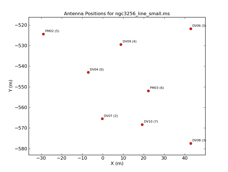
Plot Antenna Positions
This task is a simple plotting interface to produce plots of the antenna positions (taken from the ANTENNA sub-table of the MS). The location of the antennas in the MS will be plotted with X-toward local east, Y-toward local north.
The inputs to plotants are:
 #plotants :: Plot the antenna distribution in the local reference frame:
vis              =   ''       #Name of input visibility file (MS)
figfile          =   ''       #Save the plotted figure to this file
antindex         =   False    #Label antennas with name and antenna ID
logpos           =   False    #Whether to plot logarithmic positions
exclude          =   ''       #Antenna name/id selection to exclude from plot
checkbaselines   =   False    #Whether to check baselines in the main table.
title            =   ''       #Title for the plot.
showgui          =   True     #Show plot on gui.
For most telescopes, the default X/Y plot is in meters. For VLBA antenna plots, latitude vs. longitude (degrees) is plotted instead.
Supported format extensions for the figfile include emf, eps, pdf, png, ps, raw, rgba, svg, and svgz, depending on which python modules are installed on your system. Formats currently available in a downloaded CASA package include all but emf (enhanced metafile).
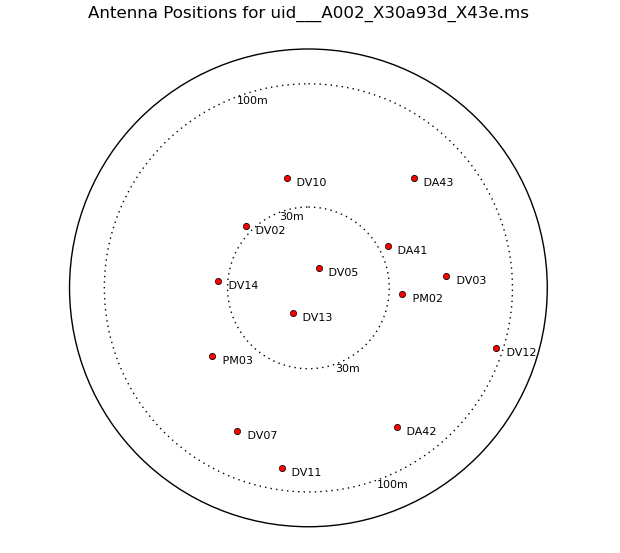
Each antenna position is labeled with the antenna name. VLBA antenna plots label the positions with “name @ station” format, e.g. “2@FD” for the Fort Davis, Texas, antenna. To add the antenna ID to the name, set antindex=True as shown in Figure 1.
ALMA antenna positions with antindex=True.
By default, plotants plots the positions of all antennas in the ANTENNA subtable. However, the user has the option to exclude certain antennas with the exclude parameter. Its value is a string to select which antennas to exclude, using the same syntax as the antenna parameter in MeasurementSet selection. For example, exclude=”5~6” would exclude the PM antennas from the plot in Figure 1.
To plot only those antennas which appear in the MAIN table (e.g. after a split, which retains the entire ANTENNA subtable in the dataset), set checkbaselines=True. This parameter would have automatically removed antenna 7 (DV10) from the plot in Figure 1, as it does not appear in the main table of this dataset.
To plot logarithmic positions instead of X/Y positions, set logpos=True as shown in Figure 2:
Antenna positions with logpos=True
The default title for the plot is “Antenna Positions for ” the MS name (vis argument), as shown in all figures on this page. To set a custom title, set the title parameter to the desired string.
The plotants GUI
By default, the plotants GUI will be shown when the task is used. If the GUI is not needed, as in scripting mode to produce a figfile, set showgui=False. When casa flags are set to avoid starting GUI tools or to run without the matplotlib ‘tkagg’ backend (–nogui, –pipeline, or –agg), the plotants GUI will not be shown regardless of the value of the showgui parameter.
The antennas will be plotted in a plotter window as shown below. Several tool buttons are available to manipulate and save the plot:
The ‘Home’ button (leftmost house icon) is used to return to the first, default view after panning or zooming.
The ‘Forward’ and ‘Back’ buttons (left- and right-arrow icons) are used to navigate between previous plot views after pan/zoom actions.
The ‘Pan/Zoom’ button (crossed blue arrows, fourth icon) is used to drag the plot to a new position by pressing and holding the mouse button.
The ‘Zoom-to-rectangle’ button (magnifier icon, fifth from left) is used to mark a rectangular region with the mouse in order to zoom in on the plot.
The ‘Subplot-configuration’ button (sixth icon) can be used to stretch or compress the left, right, top, or bottom of the plot, as well as the ability to reset the plot to the original shape after manipulation before exiting the configuration dialog.
The ‘Save’ button (rightmost icon) is used to export the plot. A file save dialog is launched to select a location, name, and format (default png) for the file.
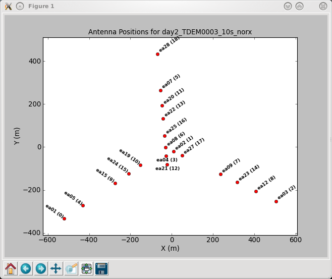
plotants GUI for a VLA dataset with antindex=True. Note the tool buttons at the bottom of the window.
VLA Weather Information
Weather data for the VLA can be displayed with the task plotweather. This task will also calculate opacities based on the weather data taken at the time of the observation, or from a seasonal model.
Inputs are:
#plotweather :: Plot elements of the weather table; estimate opacity.
vis = ''              #MS name
seasonal_weight = 0.5 #weight of the seasonal model
doPlot = True         #set this to True to create a plot
plotName = ''         #(Optional) the name of the plot file
The amount of seasonal data can be set by the parameter seasonal_weight, where a value of 1 will only use the seasonal model and a value of 0 will only use the actual weather data to calculate opacities.
Typical output of plotweather looks like below:
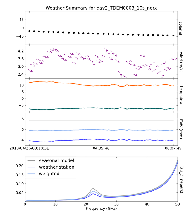
Typical output from plotweather. The panel at the top displays the following properties as a fiunction of time across the observation: elevation of the sun, wind speed and direction, temperature and dew point, and precipitable water vapor (pwv). The bottom panel shows the calculated zenith opacity as a function of frequency. The opacities calculated from the actual weather data, from a seasonal model and the specified mix of both are shown in the PWV and Tau plots.
The methods used in this task are described EVLA Memo 143, VLA Test Memo 232, and VLA Scientific Memo 176. The wind direction aligns with the meteorological definition, i.e., north is up (0deg) with the angle increasing clockwise E, S, W (e.g., a vector pointing to the right indicates westerly winds with an angle of 270deg).
Allowed output plot formats are those supported by matplotlib, currently emf, eps, pdf, png, ps, raw, rgba, svg, and svgz.
Alert: plotweather accesses the WEATHER table in the MS. The task may therefore also work for non-VLA data as long as such a table is present. The plots and calculations, however, have been tailored for the VLA, so non-VLA data may or may not be interpreted correctly.
Browse MS/Calibration Tables
The browsetable task is available for viewing data directly. It handles all CASA tables, including MeasurementSets, calibration tables, and images. This task brings up a CASA Qt table browser, which can be launched from outside CASA using casabrowser.
browsetable is not required for normal data reduction but is useful for troubleshooting or for identifying table column names and formats. If you want to edit a long column or extract data for manipulation outside CASA (e.g. the uv data), see flagdata and the table tools in the Global Tool List. The MeasurementSet columns and subtables are described here.
For CASA 6, inp/go no longer works with browsetable, and browsetable should be invoked using the argument:
browsetable('ngc5921_ut.ms')
Available sub-parameters are given on the browsetable task pages.
For an MS, as in this example, the table browser will display the MAIN table (Figure 1). To look at subtables, use the table keywords tab along the left side to bring up a panel with the subtables listed (Figure 2), then choose (double-click) a table name (Keyword) to display the subtable in a new tab (Figures 3 and 4). You can double-click on a cell in a table to view the contents (fourth figure below) then use the “Close” or “Close All” buttons at the bottom of the contents display to close one or all displayed values.

The browser displays the MAIN table within a frame. You can scroll through the data with the sliders at right and bottom, and step through the pages with the “<<” and “>>” buttons or using “First” and “Last” to quickly advance to the beginning or end. To go to a specific page, input the page number in the text box then click “Go”. By default, 1000 rows of the table are loaded at a time, but you can specify this setting in the “Loading … rows” text box.
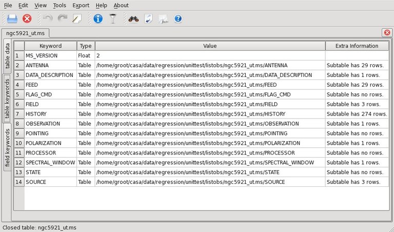
Use the “table keywords” tab to look at other tables within an MS. Double-click on a table name to view its contents in a new tab, as shown in the following figures.
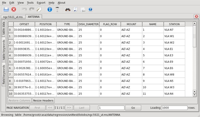
Viewing the ANTENNA table of the MS.
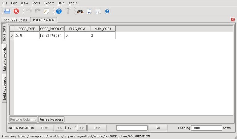
The POLARIZATION table shows the number and types of correlations. The CORR_TYPE integer array indicates the Stokes type as defined in the Stokes class enumeration. Common types include RR (5), RL (6), LR (7), and LL (8) for circular polarization, and XX (9), XY (10), YX (11), and YY (12) for linear polarization.
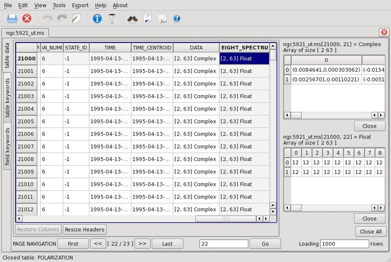
Double-click a cell in the table or sub-table to see its value displayed to the right. Here, the DATA column cell (top right) contains a [2,63] array of complex numbers. The WEIGHT_SPECTRUM for this data is shown below it as a [2,63] array of float values. Use the sliders to see other values in the arrays, and click “Close” to close the cell contents display or “Close All” to close all contents displays.
Many options are available on the browsetable toolbar and menus:
To open a table, click the “Open Table” button or use the File > Open Table menu to open a file browser dialog box.
To close a table, click the “Close Table” button to close the table in the active tab, or use the options on the “File” menu to close the table in the active tab (“Close Table”), to select an open table to close (“Close…”), or to close all tables (“Close All”). You can also “Close All and Exit” the table browser.
To edit the table and its contents, click the “Edit Table” button or use the Edit > Edit Table menu. You can also use the “Edit**”** menu to add a row to the table. Be careful with this, and make a backup copy of the table before editing!
To view table information, click the “Table Information” (blue *”i”* button) or use the View > Table Information menu. You can also hover the mouse pointer over the table name tab to get a popup with information.
To set a TaQL filter, click the “Filter on Fields” button or use the View > Filter on Fields menu. This will open a “Filter Rules” dialog box within the table browser in which to set the filter. Another option is to use the taql parameter in the browsetable() call.
To choose which columns to display, use View > Columns to select the columns from a list, which you can select individually or toggle with “Show All Columns” or “Hide All Columns”. Another option is to use the skipcols parameter in the browsetable() call.
To format the contents of the column cells, use View > Format Display to select a column then choose its formatting (depending on its type). For example, for numerical values you can set the precision and choose to use scientific format, or set the font and color for negative and nonnegative values.
To find data using filter rules, click the “Find” button or use Tools > Find to open a Search Rules dialog box.
To sort the table, click the “Sort” button, use the Tools > Sort menu to open a Table Sorter dialog box in which you can select the sort columns,or just click on the column name. Another option is to use the sortlist parameter in the browsetable() call.
To plot table data, click the “Plot 2D” button or use the Tools > Plot 2D menu to open a Plot Options dialog box where you can select the rows and axes to plot, along with plot display options. Click “Overplot” or “Clear and Plot” to make the plot in the Table Browser Plotter window. There is also an option to export the plot; select PNG or JPG format and click Go.
Currently, Export > VOTable results in a Fatal IO Error and kills the table browser.
The default display is 1000 rows, but this can be set in the input box at the lower right. To page through the table, use the PAGE NAVIGATION buttons to advance forward or backward one page, or go directly to the First or Last page. You can also enter a page number and click Go.
To exit the table browser, use File > Exit or click the Close “X” button at the upper right of the window.
Alert: You are likely to find that browsetable needs to get a table lock before proceeding. Use the clearstat command to clear the lock status in this case. You may also be unable to use other tasks on the table while it is open in the table browser.
Plot/Flag Visibilities
A number of CASA tasks handle the plotting and flagging of visibilities. The following subsections describe the usage of the relevant tasks:
plotms — create X-Y plots of data in MS and calibration tables, flag data
flagdata — data flagging
flagcmd — manipulate and apply flags using FLAG_CMD table
flagmanager — manage versions of data flags
msview — two-dimensional viewer used for manipulating visibilities
Plot/Edit using plotms
plotms is a GUI-style plotter, based on Qt, for creating X-Y plots of visibility data and calibration tables. It can either be started as a task within CASA or from outside CASA (type casaplotms on the command line). This task also provides editing capability.
plotms was originally intended to plot MeasurementSets (the “ms” in “plotms”) but has been extended to include calibration tables. Supported cal table types include B Jones, B TSYS, BPOLY, D Jones, Df Jones, DfLLS Jones, EGainCurve, F Jones, Fringe Jones, G Jones, GlinXphf Jones, G EVLASWPOW, GSPLINE, K Jones, KAntPos Jones, Kcross Jones, T Jones, TOpac, Xf Jones, A Mueller, M Mueller, and SDSKY_PS (single-dish sky calibration). Some axis choices do not apply to calibration tables, and the calibration axes do not apply to MeasurementSets. Selection can be applied to calibration tables; where relevant, channel selection has been implemented and tested for the cal tables listed. Averaging cannot be used for BPOLY and GSPLINE tables, which use an older table format. Some options, such as certain axes and transformations, have not been implemented yet for calibration tables.
For simplicity, this document primarily addresses plotting MeasurementSets.
The current inputs and default values for plotms include:
plotms :: A plotter/interactive flagger for visibility data.
vis                 =         ''        # input MS or CalTable (blank for none)
gridrows            =          1        # number of subplot rows (default 1).
gridcols            =          1        # number of subplot columns (default 1).
rowindex            =          0        # row location of the plot (0-based, default 0)
colindex            =          0        # column location of the plot (0-based, default 0)
plotindex           =          0        # index to address a subplot (0-based, default 0)
xaxis               =         ''        # plot x-axis (blank for default/current)
yaxis               =         ''        # plot y-axis (blank for default/current)
selectdata          =       True        # data selection parameters
     field          =         ''        # field names or field index numbers (blank for all)
     spw            =         ''        # spectral windows:channels (blank for all)
     timerange      =         ''        # time range (blank for all)
     uvrange        =         ''        # uv range (blank for all)
     antenna        =         ''        # antenna/baselines (blank for all)
     scan           =         ''        # scan numbers (blank for all)
     correlation    =         ''        # correlations/polarizations (blank for all)
     array          =         ''        # (sub)array numbers (blank for all)
     observation    =         ''        # observation ID(s) (blank for all)
     intent         =         ''        # observing intent (blank for all)
     feed           =         ''        # feed (blank for all)
     msselect       =         ''        # MS selection (blank for all)
averagedata         =       True        # data averaging parameters
     avgchannel     =         ''        # average over channel (blank = False, otherwise value in channels)
     avgtime        =         ''        # average over time (blank = False, other value in seconds)
     avgscan        =      False        # average over scans if time averaging is enabled
     avgfield       =      False        # average over fields if time averaging is enabled
     avgbaseline    =      False        # average over all baselines  (mutually exclusive with avgantenna)
     avgantenna     =      False        # average by per-antenna  (mutually exclusive with avgbaseline)
     avgspw         =      False        # average over all spectral windows
     scalar         =      False        # do scalar averaging
transform           =      False        # transform data in various ways
extendflag          =      False        # extend flagging to other data points
iteraxis            =         ''        # axis over which to iterate
customsymbol        =      False        # set a custom symbol for unflagged points
coloraxis           =         ''        # set data axis to use for colorizing
customflaggedsymbol =      False        # set a custom plot symbol for flagged points
xconnector          =          ''       # set connector for data points (blank="none"; "line","step")
plotrange           =         []        # plot axes ranges: [xmin,xmax,ymin,ymax]]
title               =         ''        # title written along top of plot
titlefont           =          0        # font for plot title
xlabel              =         ''        # text for horizontal axis. Blank for default.
xaxisfont           =          0        # font for plot x-axis
ylabel              =         ''        # text for vertical axis. Blank for default.
yaxisfont           =          0        # font for plot y-axis
showmajorgrid       =      False        # show major grid lines (horiz and vert.)
showminorgrid       =      False        # show minor grid lines (horiz and vert.)
showlegend          =      False        # show a legend on the plot
plotfile            =         ''        # name of plot file to save automatically
showgui             =       True        # show GUI
clearplots          =       True        # remove any existing plots (do not overplot)
callib              =       ['']        # calibration library string or filename for on-the-fly calibration.
headeritems         =         ''        # comma-separated list of pre-defined page header items
showatm             =      False        # compute and overlay the atmospheric transmission curve
showtsky            =      False        # compute and overlay the sky temperature curve
showimage           =      False        # compute and overlay the image sideband curve.
Note that when some parameters are set or are True, their subparameters are displayed by inp( ). By default, selectdata, averagedata, and showgui are True and their subparameters are shown above. Other parameters with subparameters include:
xaxis                     =        'real'  # plot x-axis (blank for default/current)
     xdatacolumn          =            ''  # data column for x-axis (blank for default/current)
yaxis                     =        'imag'  # plot y-axis (blank for default/current)
     ydatacolumn          =            ''  # data column for y-axis (blank for default/current)
     yaxislocation        =        'left'  # set yaxis to the left of the plot
transform                 =          True  # transform data in various ways?
     freqframe            =            ''  # frame in which to render frequency and velocity axes
     restfreq             =            ''  # rest frequency to use for velocity conversions
     veldef               =       'RADIO'  # definition in which to render velocity
     shift                =    [0.0, 0.0]  # adjust phases by this approximate phase center shift [dx,dy] (arcsec)
extendflag                =          True  # extend flagging to other data points
     extcorr              =         False  # extend flags based on correlation
     extchannel           =         False  # extend flags based on channel
iteraxis                  =    'baseline'  # axis over which to iterate
     xselfscale           =         False  # use common x-axis range (scale) for iterated plots
     yselfscale           =         False  # use common y-axis range (scale) for iterated plots
     xsharedaxis          =         False  # enable iterated plots on a grid to share a common external x-axis per column
     ysharedaxis          =         False  # enable iterated plots on a grid to share a common external y-axis per row
customsymbol              =          True  # set a custom symbol for unflagged points
     symbolshape          = 'autoscaling'  # shape of plotted unflagged symbols
     symbolsize           =             2  # size of plotted unflagged symbols
     symbolcolor          =      '0000ff'  # color of plotted unflagged symbols
     symbolfill           =        'fill'  # fill type of plotted unflagged symbols
     symboloutline        =         False  # select outlining plotted unflagged points
customflaggedsymbol       =          True  # set a custom plot symbol for flagged points
     flaggedsymbolshape   =     'nosymbol  # shape of plotted flagged symbols
     flaggedsymbolsize    =             2  # size of plotted flagged symbols
     flaggedsymbolcolor   =      'ff0000'  # color of plotted flagged symbols
     flaggedsymbolfill    =        'fill'  # fill type of plotted flagged symbols
     flaggedsymboloutline =         False  # select outlining plotted flagged points
showmajorgrid             =          True  # show major grid lines (horiz and vert.)
     majorwidth           =             0  # line width in pixels of major grid lines
     majorstyle           =            ''  # major grid line style: solid dash dot none
     majorcolor           =            ''  # color of major grid lines as name or hex code
showminorgrid             =          True  # show minor grid lines (horiz and vert.)
     minorwidth           =             0  # line width in pixels of minor grid lines
     minorstyle           =            ''  # minor grid line style: solid dash dot none
     minorcolor           =            ''  # color of minor grid lines as name or hex code
plotfile                  =    'plot.jpg'  # name of plot file to save automatically
     expformat            =            ''  # export format type (jpg, png, ps, pdf, txt), else use plotfile extension
     verbose              =          True  # include metadata in text export
     exprange             =            ''  # export all iteration plots or only the current one
     highres              =         False  # use high resolution
     dpi                  =            -1  # DPI of exported plot
     width                =            -1  # width of exported plot
     height               =            -1  # height of exported plot
     overwrite            =         False  # overwrite plot file if it already exists
Note that if the vis parameter is set to the name of a MeasurementSet here, when you start plotms the entire MeasurementSet will be plotted, which can be time consuming. You may want to set selection or averaging parameters first.
To start a “blank” plotms window then enter your selections interactively in the GUI, use these commands:
default plotms
plotms
Alternatively, they can be specified as task parameters in a plotms call, for scripting:
plotms(vis1, yaxis='phase', ydatacolumn='corrected', xaxis='frequency', coloraxis='spw', antenna='1', spw='0:3~10', corr='RR', avgtime='1e8', plotfile='vis1.jpg')
Note that subsequent plotms calls will return any unspecified parameters in that call to their default values. See also the Examples tab in the plotms task for plotms calls using many of the parameters.
The plotms GUI will be described in the following sections, along with the corresponding parameters for the task interface or scripting. For non-interactive scripting, set showgui=False and export the plot into an image specified by plotfile.
The Plot Tab
Loading, Selecting, and Averaging Data: the Plot Data Tab
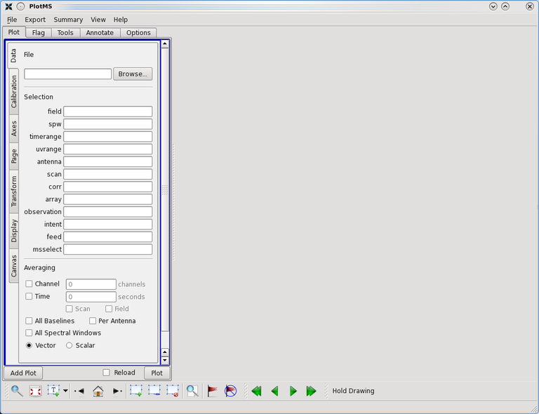
The plotms window starts on the Plot > Data tab. No parameters have been set.
File Selection
When plotms is first started, by default it will display the Plot tab (as chosen from the tabs at the top of the plotms window) and its Data subtab (as chosen from the tabs on the left side) as shown in Figure 1. First, a MeasurementSet or calibration table should be loaded by clicking on Browse in the File section and selecting a MeasurementSet directory (just select the directory itself; do not descend into it).
A plot can now be made of the MeasurementSet by clicking on the Plot button, but you may want to set selection or averaging parameters first rather than plot the entire dataset. By default, plotms will plot Amplitude versus Time for a MeasurementSet; see the Axes Tab section for axis options. The default axes change for calibration tables depending on the table type. plotms self-scales axes and the symbol size. For a very large range, this can hide points close to zero; see the Axes Tab section for setting axis ranges and the Display Tab section for setting symbol size.
The plotms task parameter for file selection is vis.
Data Selection
The options for data selection are:
field
spw
timerange
uvrange
antenna
scan
corr (correlated polarizations)
array
observation
intent
feed
msselect
Note that, unlike when setting data selection parameters from the CASA command line, no quotation marks are needed around strings in the GUI. For more information on data selection strings, see the documentation here. To view information about your data in order to make your selection, use the Summary menu or the listobs task.
Calibration table selection may differ from MeasurementSet selection:
antenna selection for a calibration table depends on its type.
For antenna-based cal tables without a reference antenna, only ANTENNA1 is matched and the “&” operators in selection expressions are ignored. Single-dish sky calibration tables use ANTENNA1 selection.
For antenna-based cal tables with a reference antenna, ANTENNA2 is interpreted as a reference antenna and matched against the ANT2 in “ANT1&ANT2” type expressions. “ANT” selections continue to match ANTENNA1 only.
For baseline-based cal tables, antenna selection uses both ANTENNA1 and ANTENNA2 as described in the MSSelection documentation.
corr selection is used to select calibration table polarizations, including “/” for a ratio plot.
The plotms task parameter for data selection is selectdata (default is True, but no selection occurs unless one or more subparameters is set). Its subparameters include field, spw, timerange. uvrange, antenna, scan, correlation, array, observation, intent, feed, and msselect. These should be set to string values.
Averaging Data
plotms enables averaging of the data in order to increase signal-to-noise of the plotted points or to increase plotting speed.
Averaging is currently not supported for Ant-Ra and Ant-Dec axes and will result in a warning in the log, then the unaveraged data will be plotted.
Averaging is supported for calibration tables with the exception of BPOLY and GSPLINE tables, which use an older table format.
The options for averaging in the Plot > Data tab include:
channel
time (optionally over scans or fields)
all baselines or per antenna
all spectral windows
vector (default) or scalar
The box next to a given averaging mode needs to be checked for that averaging to take effect. The Weight and Sigma axes are not supported in some averaging modes. Note that the “average weight” is actually the weight sum accumulated when performing the average; i.e., the net weight of a weighted-averaged datum is the sum of the weights going into the average.
When averaging, plotms will prefer unflagged data. If an averaging bin contains any unflagged data at all, only the average of the unflagged will be shown. For averaging bins that contain only unflagged data, the average of that unflagged data will be shown. When flagging on a plot of averaged data, the flags will be applied to the unaveraged data in the MS.
The plotms task parameter for averaging is averagedata (default is True, but no averaging occurs unless one or more subparameters are set). It subparameters include avgchannel and avgtime (set to a string value in channels or seconds, default “”), and boolean parameters avgscan, avgfield, avgbaseline, avgantenna, avgspw, and scalar (True/False, default False). Invalid combinations of averaging will result in an error message (e.g. avgbaseline=True, avgantenna=True) or will be ignored (e.g. avgscan=True but avgtime has not been set).
Channel Averaging: to average n channels together, the user would click on the box next to Channel so that an “X” appears in it, and then type the number n in the empty box. When the user next clicks on Plot, every n channels will then be averaged together and plotted against the average channel numbers. The total number of channels plotted will be decreased by a factor of n.
Channel selection may be combined with channel averaging. For MeasurementSets, each selected channel range is binned and averaged individually, but for calibration tables, the selected channels are treated as contiguous. See examples in the plotms task channel averaging documentation.
Warning: If a complex channel selection is made e.g. of continuum in the presense of multiple lines, channel averaging is unlikely to produce a meaningful plot.
Time Averaging: Time averaging is controlled by three fields. If the checkbox next to Time is checked, a blank box with units of seconds will become active, along with two additional checkboxes: Scan and Field. If averaging is desired over a relatively short interval (say, 30 seconds, shorter than the scan length), a number can simply be entered into the blank box and, when the data are replotted, the data will be time averaged. Clicking on the Scan or Field checkbox in this case will have no impact on the time averaging. These checkboxes become relevant if averaging over a relatively long time—say the entire observation, which consists of multiple scans—is desired. Regardless of how large a number is set in the Time averaging box, only data within individual scans will be averaged together. In order to average data across scan boundaries, the Scan checkbox must be checked and the data replotted. Finally, clicking on the Field checkbox enables the averaging of multiple fields together in time.
Averaging All Baselines/Per Antenna: Clicking on the All Baselines checkbox will average all baselines in the array together. Alternatively, the Per Antenna box may be checked, which will average all baselines for a given antenna together. In this case, all baselines are represented twice; baseline 3-24 will contribute to the averages for both antenna 3 and antenna 24. This can produce some rather strange-looking plots if the user also selects on antenna—say, if the user requests to plot only antenna 0 and then averages Per Antenna, In this case, an average of all baselines including antenna 0 will be plotted, but each individual baseline including antenna 0 will also be plotted (because the presence of baselines 0-1, 0-2, 0-3, etc. trigger Per Antenna averaging to compute averages for antennae 1, 2, 3, etc. Therefore, baseline 0-1 will contribute to the average for antenna 0, but it will also singlehandedly be the average for antenna 1.) These averaging modes currently do not support the Weight and Sigma axes.
Averaging All Spectral Windows: Spectral windows can be averaged together by checking the box next to All Spectral Windows. This will result in, for a given channel n, all channels n from the individual spectral windows being averaged together. This averaging mode currently does not support the Weight and Sigma axes.
Vector/Scalar Averaging: The default mode is vector averaging, where the complex average is formed by averaging the real and imaginary parts of the relevant visibilities. If Scalar is chosen, then the amplitude of the average is formed by a scalar average of the individual visibility amplitudes.
Brief Note Regarding plotms Memory Usage
In order to provide a wide range of flexible interactive plotting options while minimizing the I/O burden and speeding up the plotting, plotms caches the data values for the plot (along with a subset of relevant meta-info) in as efficient a manner as possible. Sometimes, however, the data changes on disk, for example when other data processing tasks are applied. To force plotms to reload the data, check the Reload box next to the Plot button or press the SHIFT key while clicking the Plot button.
For plots of large numbers of points, the total memory requirement can be quite large. plotms attempts to predict the memory it will require (typically 5 or 6 bytes per plotted point when only one axis is a data axis, depending upon the data shapes involved), and will complain if it believes there is insufficient memory to support the requested plot. For most practical interactive purposes (plots that load and draw in less than a few or a few 10s of minutes), there is usually not a problem on typical modern workstations. Attempts to plot large datasets on small laptops might be more likely to encounter problems here.
The absolute upper limit on the number of simultaneously plotted points is currently set by the ability to index the points in the cache. For modern 64 bit machines, this is about 4.29 billion points (requiring around 25GB of memory). Such plots are not especially useful interactively, since the I/O and draw become prohibitive.In general, it is usually most efficient to plot data in modest chunks of no more than a few hundred million points or less, either using selection or averaging. Note that all iterations are (currently) cached simultaneously for iterated plots, so iteration is not a way to manage memory use. A few hundred million points tends to be the practical limit of interactive plotms use with respect to information content and utility in the resulting plots, especially when you consider the number of available pixels on your screen.
On-The-Fly Calibration: the Plot Calibration Tab
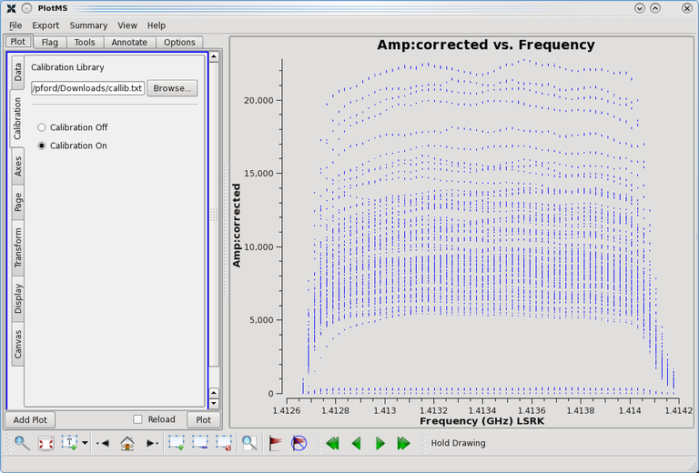
The plotms Calibration tab. This MeasurementSet has no CORRECTED_DATA column. A calibration library file was selected with the file browser and applied on the fly.
One can apply calibration tables to the uncalibrated data on the fly, i.e. without a run of applycal beforehand, by specifying a calibration library and selecting the corrected Data Column for the plotted axes. See the Cal Library Syntax documentation for more information on specifying calibration in a string or file.
The Calibration tab on the left hand side contains a field to specify a calibration library file, or use Browse to open a file selection dialog. You can also specify the calibration library commands directly in a string. There is a switch to apply the calibration library to produce the corrected data (Calibration On) or to show an existing CORRECTED_DATA column (Calibration Off). If the corrected Data Column is requested but the column is not present in the MS and the calibration library is not set or enabled, plotms issues a warning and plots the DATA column instead.
The plotms task parameter ‘callib’ can be used to provide a calibration library file or a string containing the cal library commands. It is enabled by default when the parameter is set.
Selecting Plot Axes: The Plot Axes Tab
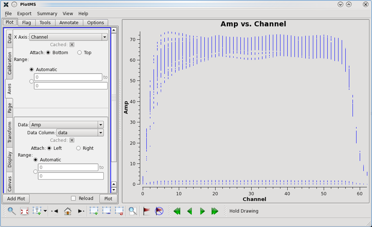
The plotms Plot > Axes tab, used here to make a plot of Amp vs. Channel.
Selecting Axes
The X and Y axes of a plot are selected by clicking on the Plot > Axes tab and choosing an entry from the drop-down menus below X Axis and Y Axis. The axes are grouped by type and listed in this order:
Visibility values and flags: - Amp — Data amplitudes in units which are proportional to Jansky (for data which are fully calibrated, the units should be in Jy). - Phase — Data phases in units of degrees. - Real and Imag — The real and imaginary parts of the visibility in units which are proportional to Jansky (for data which are fully calibrated, the units should be Jy). - Wt and **Wt*Amp**** — the weight of the visibility and the product of the weight and the amplitude. - **WtSp — WEIGHT_SPECTRUM column, i.e. a weight per channel. - Sigma — the SIGMA column of the visibilities - SigmaSp — SIGMA_SPECTRUM column, i.e. a sigma per channel - Flag — Data which are flagged have Flag = 1, whereas unflagged data are set to Flag = 0. Note that, to display flagged data, you will have to click on the Plots > Display tab and choose a Flagged Points Symbol. - FlagRow — In some tasks, if a whole data row is flagged, then FlagRow will be set to 1 for that row. Unflagged rows have FlagRow = 0. However, note that some tasks (like plotms) may flag a row, but not set FlagRow = 1. It is probably better to plot Flag than FlagRow for most applications.
Calibration: - GainAmp, GainPhase, GainReal, GainImag — the amplitude, phase, real and imaginary part of the calibration tables for regular complex gain tables. - Delay — The delay of a delay or fringefit (Fringe Jones) calibration table. - Delay Rate — The delay rate of a fringefit (Fringe Jones) calibration table. - Disp Delay — The dispersive delay of a fringefit (Fringe Jones) calibration table. - SwPower — Switched Power values for a VLA switched power calibration table. - Tsys — Tsys for Tsys calibration tables. - Opac — Opacity values of a Opacity calibration table. - SNR — Signal-to-Noise Ratio of a calibration table. - TEC — Total Electron Content of an ionosphere correction calibration table. - Antenna Positions — Antenna position offsets for a KAntPos Jones calibration table.
Ephemeris: - Radial Velocity — for an ephemeris source, in km/s. - Distance (rho) — for an ephemeris source, in km.
If the data axis selected from the drop-down menu is already stored in the cache (therefore implying that plotting will proceed relatively quickly), an “X” will appear in the checkbox next to Cached. To reload the data from disk, the Reload checkmark should be set at the bottom of this display.
The plotms task parameters used to select the axes are xaxis and yaxis. Valid options include ‘scan’, ‘field’, ‘time’, ‘interval’, ‘spw’, ‘chan’ (or ‘channel’), ‘freq’ (or ‘frequency’), ‘vel’ (or ‘velocity’), ‘corr’ (or ‘correlation), ‘ant1’ (or ‘antenna1’), ‘ant2’ (or ‘antenna2’), ‘baseline’, ‘row’, ‘observation’, ‘intent’, ‘feed1’, ‘feed2’, ‘amp’ (or ‘amplitude’), ‘phase’, ‘real’, ‘imag’, ‘wt’ (or ‘weight’), ‘wtsp’ (or ‘weightspectrum’), ‘flag’, ‘flagrow’, ‘uvdist’, ‘uvwave’ (or ‘uvdistl’), ‘u’, ‘v’, ‘w’, ‘uwave’, ‘vwave’, ‘wwave’, ‘azimuth’, ‘elevation’, ‘hourang’ (or ‘hourangle’), ‘parang’ (or ‘parangle’), ‘ant’ (or ‘antenna’), ‘ant-azimuth’, ‘ant-elevation’, ‘ant-ra’, ‘ant-dec’, ‘ant-parang’ (or ‘ant-parangle’), ‘gainamp’ (or ‘gamp’), ‘gainphase’ (or ‘gphase’), ‘gainreal’ (or ‘greal’), ‘gainimag’ (or ‘gimag’), ‘delay’ (or ‘del’), ‘delayrate’ (or ‘rate’), ‘dispdelay’ (or ‘disp’), ‘swpower’ (or ‘swp’ or ‘spgain’), ‘tsys’, ‘opacity’ (or ‘opac’), ‘snr’, ‘tec’, ‘radialvelocity’, ‘distance’ (or ‘rho’).
When left as the default empty strings (“”), the axes for a MeasurementSet will be Amp vs. Time. The default axes for a calibration table depend on the type.
Setting Axes Parameters
Data Columns: - For relevant data axes like Amp and Phase, the user will be presented with the option to plot raw data or calibrated data. This can be selected via a Data Column drop-down menu, located directly under the drop-down menu for X Axis or Y Axis selection. To plot raw data, select “data”; to plot calibrated data, select “corrected”. Note that this choice will only have an impact on a plot if a calibration table has been applied to the MeasurementSet or a calibration library is set and enabled. - If a data model is present in the MeasurementSet (e.g., created by setjy, clean, or ft), it can be plotted by selecting “model” from the Data Column menu. For MeasurementSets with float data instead of complex data, common in singledish datasets, select the “float” datacolumn. - Residuals can be plotted via “corrected-model_vector”, “corrected-model_scalar”, “data-model_vector”, data-model_scalar”, “corrected/model_vector”, “corrected/model_scalar”, “data/model_vector”, and “data/model_scalar”. The vector and scalar options distinguish between versions where values like amp, phase, etc. are calculated before (scalar) or after (vector) the subtraction or division. - The plotms task parameters used to select the data columns are xdatacolumn and ydatacolumn. Valid options include ‘data’, corrected’, ‘model’, ‘float’, ‘corrected-model’ (vector implied), ‘corrected-model_vector’, ‘corrected-model_scalar’, ‘data-model’ (vector implied), ‘data-model_vector’, ‘data-model_scalar’, ‘corrected/model’ (vector implied), ‘corrected/model_vector’, ‘corrected/model_scalar’, ‘data/model’ (vector implied), ‘data/model_vector’, and ‘data/model_scalar’. The implied vector residual datacolumns were kept for backwards compatibility. Default data columns for x and y are both ‘data’.
WARNING: plotting antennas pointing directions with the Ant-Ra / Ant-Dec axes has only been implemented for ALMA, ASTE, and NRO data.
Axis Locations
The location of the x-axis and y-axis can be set using the radio buttons in the GUI, where the x-axis can be located at the Bottom (default) or Top, and the y-axis can be located at the Left (default) or Right.
The plotms task parameter to set the y-axis location is yaxislocation. Valid values for this parameter include ‘left’ (default) and ‘right’. There is no parameter to set the x-axis location.
Axes Ranges
The X and Y ranges of the plot can be set manually or automatically. By default, the circle next to Automatic will be checked, and the ranges will be auto-scaled in ascending order based on the values plotted.
To define the range, click on the circle below Automatic and enter a minimum and maximum value in the blank boxes. Note that if identical values are placed in the blank boxes (xmin=xmax and/or ymin=ymax), then the values will be ignored and automatically set. When xmin > xmax or ymin > ymax, the tick values will be descending (reversed).
The plotms task parameter used to set the axes ranges is plotrange, and its value is a list of numbers in the format [xmin, xmax, ymin, ymax] (default [ ], automatic range).
Plotting Multiple Y-Axes
Different values of the same dataset can be shown at the same time. To add a second y-axis, press the Add Y Axis Data button at the bottom of the Axes tab. Then select the parameters for the newly created axis by selecting from the new “Y Axis Data” drop-down menu. If the two y-axes have the same units, they can be displayed both on the same axis. If they are different (or their ranges are dissimilar), e.g. Amplitude and Elevation (both versus Time; see Figure 4 below), one axis should be attached to the left and the other to the right hand side of the plot. Using more than a single y-axis data is also reflected in the Display tab where a drop-down menu appears in order to select multiple y-axis options; here you may colorize each axis differently. See the Plot Display Tab section below to learn more about symbol properties. To remove the additional y-axis, click Delete Y Axis Data at the bottom of the Axes tab.

Overplotting in plotms: Two different y-axes for the same dataset have been chosen for this plot, amplitude and elevation.
The plotms task parameters used to plot multiple y-axes are the same as for a single y-axis: yaxis and yaxislocation; multiple y-axes can be specified as a list of strings if you are specifying the plotms command in the terminal. The values for yaxis and yaxislocation should be set to lists of the same length:
plotms(vis='ngc5921.ms', yaxis=['amp','elevation'], yaxislocation=['left','right'])
Atmospheric Curve Overlays
The ability to compute and overlay an atmospheric transmission curve or a sky temperature curve, available in plotbandpass, has been added to plotms. For this feature, the x-axis must be Channel or Frequency; if another axis is chosen, a warning is issued and the plot continues without the overlay.
plotms uses the dataset’s subtables to compute the mean weather values: pressure, humidity, temperature, and precipitable water vapor (pwv). If these subtables are not found, reasonable defaults are used instead and reported in a log message. The atmosphere tool is then used by plotms to calculate dry and wet opacities to produce the requested overlay curve, corrected by the airmass based on elevation.
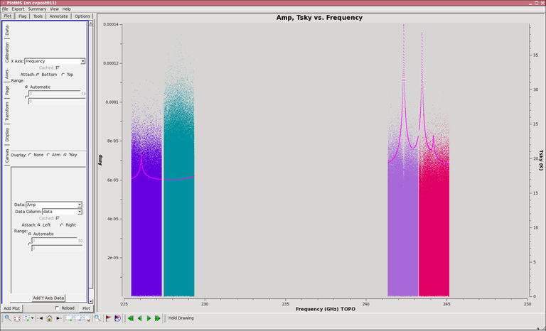
Amp vs. Frequency plot with a Tsky overlay. The Tsky y-axis is automatically added on the right, and the curve is plotted in magenta. The Plot > Axes tab shows the radio buttons to select the Overlay: None, Atm, or Tsky.
The plotms task parameters used to plot the overlays are showatm and showtsky. These take boolean values and their defaults are False. Only one overlay can be selected; if both are set to True, only the atmospheric curve (showatm) will be displayed.
plotms(vis=myvis, yaxis='amp', xaxis='freq', showatm=True)
The image sideband curve may also be shown in plotms when the atmospheric transmission or sky temperature curves are plotted. In order to do this, the MS (or associated MS for a calibration table) cannot have reindexed spectral window IDs as a result of a split, and must have an ASDM_RECEIVER table in order to read the LO frequencies. If these conditions are not met, a warning is issued and only the atm/tsky curves are calculated and plotted.
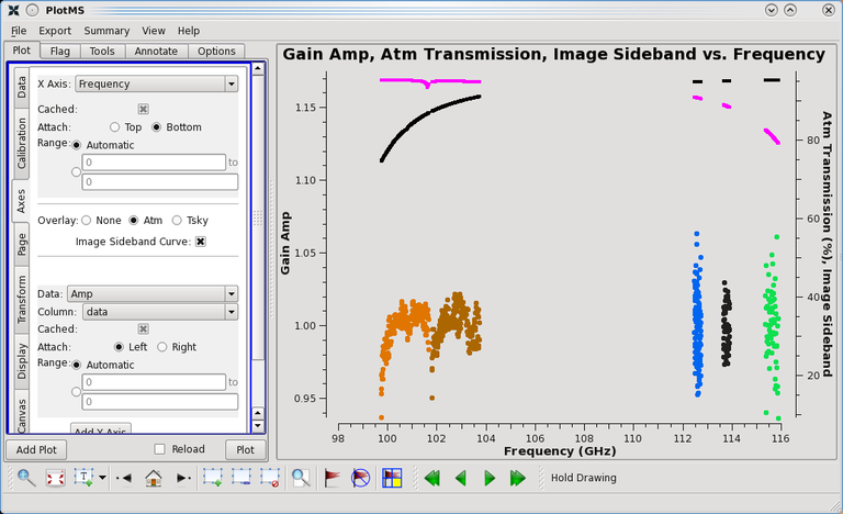
Gain Amp vs. Frequency plot for a bandpass calibration table with the Atm Transmission (magenta) and Image Sideband (black) overlays, colorized by spw and one antenna selected. The Plot > Axes tab shows the checkbox to select the image sideband curve, enabled only when the Overlay is Atm or Tsky.
The plotms task parameter used to plot the image sideband curve overlay is showimage. This takes a boolean value and its default is False. If showatm=False and showtsky=False, a warning is issued and the curve will not be calculated and plotted.
plotms(vis=mycaltable, yaxis='amp', xaxis='freq', antenna='0',
       coloraxis='spw', showatm=True, showimage=True)
Iteration and Page Header : The Plot Page Tab
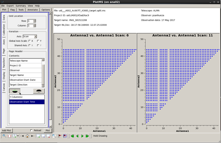
The plotms Plot Page Tab, used to iterate by scan with a page header added. The scan number is appended to the plot title.
Iteration
In many cases, it is desirable to iterate through the data that were selected in the Data tab. A typical example is to display a single baseline in an amplitude vs. time plot and then proceed to the next baselines step by step. This can be done via the Plot > Page tab. A drop-down menu allows you to select the iteration axis, with options None, Scan, Field, Spw, Baseline, Antenna, Time, and Corr. Press the Plot button after changing your selection. Each plot will be autoscaled according to its iteration value range unless a Range is specified in the Axis tab.
The current iteration is indicated in the plot title of the displayed plot. To proceed to the next plot use the green arrow buttons below the main panel. Use the icons to proceed panel by panel (single arrow symbols) or to jump to the first or last panel directly (double arrow symbols).
The number of plots per page can be selected under Options > Grid, the last of the top row of tabs, as described in the Options Tab section. There are two scaling options for the iterated axes in a grid, set in this tab: Global and Shared. Global will use a common axis range based on data loaded with the selection criteria specified in the Data tab. Shared displays one set of x-axes and y-axes for the page rather than per-plot. When left unchecked, Global and Shared results in plots with axes scaling to the data for each individual panel of the iteration. An example of global shared x-axes and y-axes is in the Options Tab section.
The plotms task parameter used to select an iteration axis is iteraxis. The options include ‘scan’, ‘field’, ‘spw’, ‘baseline’, ‘antenna’, ‘time’, and ‘corr’.
To use a global axis range for iterated plots, set parameters xselfscale=True and/or yselfscale=True. To use a shared external x-axis per column on a grid, set xsharedaxis=True (must also set xselfscale=True and gridrows greater than 1). To use a shared external y-axis per row on a grid, set ysharedaxis=True (must also set yselfscale=True and gridcols greater than 1).
Page Header
It is sometimes useful to display above the plots a page header showing some metadata information. To do so, select in the lower list the header items you want to display, and press the antenna-shaped “arrow” pointing up. This will move the items you selected to the upper list showing the header contents, without updating the page header. Multiple items can be selected at once by pressing the Shift or the Control key, Control+A selects all items. To remove items from the Contents list, select in that list the items to remove and press the antenna-shaped “arrow” pointing down. The arrows blink red when clicked while their corresponding selection is empty, green otherwise.
Press the Plot button to update the page header. Items included in the Contents list are laid out on 2 columns in the page header, in “Z” order. The contents of the header is common to all pages.
Header items from multiple plots can be displayed in the page header. In that case items from the first plot are laid out first, items from the second plot are then laid out starting from the first empty row, and so on.
The plotms task parameter used to specify header items is headeritems. The value is a single string whose value can be any comma-separated combination of the following pre-defined keywords:
‘filename’, ‘projid’, ‘telescope’, ‘observer’,’obsdate’, ‘obstime’, ‘targname’, ‘targdir’, ‘ycolumn’
When selected data leaves room for multiple candidates (e.g when selected data spans multiple observations or include multiple fields or sources), the first selected row in MeasurementSet’s Main table is used as a starting point for looking up a single “first” candidate in MeasurementSet’s auxiliary tables.
Observation Start Date and Observation Start Time are looked up in MeasurementSet’s Observation table, and therefore differ from the output of listobs task.
Transforming the Velocity Frame or Phase Center: The Plot Transform Tab
Frequency Frame
If the user plans to plot frequency, the reference frame must be defined. By default, plotms selects the frame keyword (if any) present in the data, usually the frame observed at the telescope unless modified during previous processing. However, transformations can be made by choosing a Frame from the drop-down menu in the Plot > Transform tab. Frequency reference frames can be chosen to be:
LSRK — local standard of rest (kinematic)
LSRD — local standard of rest (dynamic)
BARY — barycentric
GEO — geocentric
TOPO — topocentric
GALACTO — galactocentric
LGROUP — local group
CMB — cosmic microwave background dipole
The plotms task parameter used to select frequency frame is freqframe. Valid options include those listed above (strings with all caps). The default empty string “” results in no frame transformation.
Velocity
If Velocity is selected as an axis, by default the transformation from frequency uses the parameters in the MS metadata, or, if absent, using the central frequency and TOPO frame. The user can change this by using the Frame, Velocity Defn, and Rest Freq options in the Transform tab. The velocity definition is chosen from the Velocity Defn drop-down menu, offering selections of Radio, True (Relativistic), or Optical.
For more information on frequency frames and spectral coordinate systems, see the paper by Greisen et al. (A&A, 446, 747, 2006) (Also at http://www.aoc.nrao.edu/~egreisen/scs.ps)
Finally, the spectral line’s rest frequency in units of MHz should be typed into the Rest Freq input box next. You can use the slsearch task to search a spectral line table, or the Measures tool me.spectralline method to turn transition names into frequencies:
CASA <16>: me.spectralline('HI')
[ Out[17]: ]
{'m0': {'unit': 'Hz', 'value': 1420405751.786},
 'refer': 'REST',
 'type': 'frequency'}
For a list of known lines in the CASA measures system, use the toolkit command me.linelist(). For example:
CASA <21>: me.linelist()
[ Out[21]: 'HI H186A H185A H184A H183A H182A H181A H180A H179A H178A H177A H176A H175A ]
H174A H173A H172A H171A H170A H169A H168A H167A H166A H165A H164A H163A H162A H161A H160A...
He182A He181A He180A He179A He178A He177A He176A He175A He174A He173A He172A He171A He170A
He169A He168A He167A He166A He165A He164A He163A He162A He161A He160A He159A He158A He157A...
C186A C185A C184A C183A C182A C181A C180A C179A C178A C177A C176A C175A C174A C173A C172A
C171A C170A C169A C168A C167A C166A C165A C164A C163A C162A C161A C160A C159A C158A C157A...
NH3_11 NH3_22 NH3_33 NH3_44 NH3_55 NH3_66 NH3_77 NH3_88 NH3_99 NH3_1010 NH3_1111 NH3_1212
OH1612 OH1665 OH1667 OH1720 OH4660 OH4750 OH4765 OH5523 OH6016 OH6030 OH6035 OH6049 OH13433
OH13434 OH13441 OH13442 OH23817 OH23826 CH3OH6.7 CH3OH44 H2O22 H2CO4.8 CO_1_0 CO_2_1 CO_3_2
CO_4_3 CO_5_4 CO_6_5 CO_7_6 CO_8_7 13CO_1_0 13CO_2_1 13CO_3_2 13CO_4_3 13CO_5_4 13CO_6_5
13CO_7_6 13CO_8_7 13CO_9_8 C18O_1_0 C18O_2_1 C18O_3_2 C18O_4_3 C18O_5_4 C18O_6_5 C18O_7_6
C18O_8_7 C18O_9_8 CS_1_0 CS_2_1 CS_3_2 CS_4_3 CS_5_4 CS_6_5 CS_7_6 CS_8_7 CS_9_8 CS_10_9
CS_11_10 CS_12_11 CS_13_12 CS_14_13 CS_15_14 CS_16_15 CS_17_16 CS_18_17 CS_19_18 CS_12_19
SiO_1_0 SiO_2_1 SiO_3_2 SiO_4_3 SiO_5_4 SiO_6_5 SiO_7_6 SiO_8_7 SiO_9_8 SiO_10_9 SiO_11_10
SiO_12_11 SiO_13_12 SiO_14_13 SiO_15_14 SiO_16_15 SiO_17_16 SiO_18_17 SiO_19_18 SiO_20_19
SiO_21_20 SiO_22_21 SiO_23_22'
The plotms task parameters used to set velocity definition and rest frequency are veldef and restfreq. Valid options for veldef are ‘RADIO’, ‘TRUE’, or ‘OPTICAL’ (default is ‘RADIO’). restfreq should be in a string in MHz, for example ‘22235.08MHz’.
Shifting the Phase Center
The plot’s phase center can be shifted in the Plot > Transform tab. This will allow coherent vector averaging of visibility amplitudes far from the phase tracking center. Enter the X and Y shifts in units of arcseconds in the dX and dY boxes under Phase center shift.
The plotms task parameter used to shift the phase center is shift. Its value should be a list in the format [dx,dy] in arcsec (default [0.0, 0.0]).
Display Options for Plots: The Plot Display Tab
Colorizing Your Data
Data points can be given informative symbol colors using the Colorize option in the Plot > Display tab. By checking the box next to Colorize and selecting a data axis from the drop-down menu, the data will be plotted with colors that vary along that axis. For example, if “corr” is chosen from the Colorize menu, “RR”, “LL”, “RL”, and “LR” data will each be plotted with a different color. Note that Colorize while plotting flagged data will override the default flagged red symbol color.
The plotms task parameter used to colorize data is coloraxis. Options include ‘scan’, ‘field’, ‘spw’, ‘antenna1’, ‘antenna2’, ‘baseline’, ‘channel’, ‘corr’, ‘time’, ‘observation’, and ‘intent’.
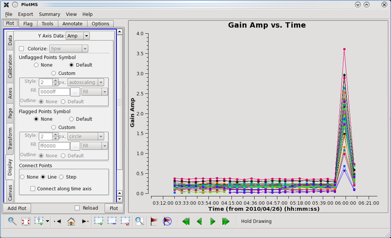
Customizing Your Symbols
Unflagged and flagged plot symbols can be customized in the Plot > Display tab. Most fundamentally, the user can choose to plot unflagged data and/or flagged data. By default, unflagged data is plotted (the circle next to Default is selected under Unflagged Points Symbol), and flagged data is not plotted (the circle next to None is selected under Flagged Points Symbol). We note here that plotting flagged data on an averaged plot is undertaken at the user’s own risk, as the distinction between flagged points and unflagged points becomes blurred if data are averaged over a dimension that is partially flagged. Take, for example, a plot of Amplitude vs. Time where all channels are averaged together, but some channels have been flagged due to RFI spikes. In creating the average, plotms will skip over the flagged channels and only use the unflagged ones. The averaged points will be considered unflagged, and the flagged data will not appear on the plot at all.
Symbol options include:
None — no data points
Default — data points which are small circles (blue for unflagged data and red for flagged data)
Custom — allows the user to define a plot symbol
If Custom plot symbols are chosen, the user can determine:
Size, by typing a number in the blank box next to px or by clicking on the adjacent up or down arrows.
Shape, chosen from the drop-down menu; options include circle, square, diamond, pixel, or autoscaling. * Note that pixel only has one possible size. *autoscaling attempts to adjust the size of the points from dots to circles of different sizes, depending on how many points are plotted.* *
Color, chosen by typing a hex color code in the Fill input box or by clicking on the … button and selecting a color from the pop-up GUI.
Fill, using the adjacent drop-down menu for how heavily the plot symbol is shaded with this color, from heaviest to lightest; options include fill, mesh1, mesh2, mesh3, and no fill.
Outline, by selecting None (no outline) or *Default *(outlined in black)
Note that if “no fill” and Outline: None are selected, the plot symbols will be invisible.
The plotms task parameter and subparameters used to customize unflagged symbols include:
customsymbol (True/False, default False) - must be True for subparameters to take effect
symbolshape (‘autoscaling’, ‘circle’, ‘square’, ‘diamond’, ‘pixel’, ‘nosymbol’, default ‘autoscaling’)
symbolsize (in number of pixels, default 2)
symbolcolor (RGB hex code e.g. ‘aa55ff’ or string color name e.g. ‘purple’, default ‘0000ff’ blue)
symbolfill (‘fill’, ‘mesh1’, ‘mesh2’, ‘mesh3’, ‘no fill’, default ‘fill’)
symboloutline (True/False, default False)
The plotms task parameters used to customize flagged symbols include customflaggedsymbol (default False) with subparameters flaggedsymbolshape (default ‘nosymbol’), flaggedsymbolsize (default 2), flaggedsymbolcolor (default ‘ff0000’ red), flaggedsymbolfill (default ‘fill’), and flaggedsymboloutline (default False). Supported values are the same as for unflagged symbols.
Symbols for Multiple Y-Axes
If you have added an additional y-axis in the Plot > Axes tab, you may customize each y-axis individually by selecting the axis in the Y Axis Data pull-down menu at the top of the Plot > Display tab and then customizing the symbols for that axis.
To set multiple symbols in the plotms task, set the symbol parameters as a list:
plotms(vis='ngc5921.ms', yaxis=['amp','elevation'], yaxislocation=['left','right'],
       customsymbol=[True,True], symbolcolor=['purple','green'])
In this plot, the ‘amp’ axis will be purple, and the ‘elevation’ axis will be green.
Connecting the Points
Plotms has the capability to connect points for calibration tables; support for MeasurementSets will be added later. The points are colorized and connected along the x-axis or time axis by line or step. Points with the same metadata but varying values of the x-axis or time are connected. Unflagged points are not connected to flagged points, even when they are not displayed. The Colorize axis will override the connection colorization.
Plot Display tab showing the Connect Points options for a gain table. Here, points with the same spw, channel, polarization, and antenna1 are connected along the time axis.
The plotms task parameters used to connect points in a calibration table plot are xconnector (default “none”, options “line” or “step”) and timeconnector (default False, or True to connect along the time axis instead of x-axis).
For an antenna position (KAntPos Jones) calibration table, the x, y, z antenna positions are located in the first axis of the data, normally the correlation axis. To distinguish these offsets, set coloraxis=’corr’ or xconnector=’line’ as shown in the figure below. To determine which points are x, y, and z, use the Locate tool.
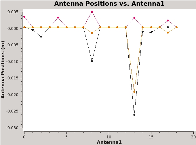
Plot Display tab showing the Connect Points options for an antenna position table.
Plot Labels: The Plot Canvas Tab
Plot Title
Options to change the plot title include None (no title), Default, and a user-input string. To set the plot title, under Title, click on the circle next to the input box and enter the desired text. This text box shows the grayed-out default string, “%%yaxis%% vs. %%xaxis%%” (to substitute the axis names for “yaxis” and “xaxis”). The user can also choose the size of the title font by checking the Title Font checkbox and entering the font size or using the arrows to increase or decrease the value. The default is to scale the title font depending on the plot size.
The plotms task parameters used to set the title and its font are title (default empty string “” for yaxis vs. xaxis) and titlefont (default 0 to autoscale). Set a space ” ” for no title.
Legend
A plot symbol legend can be added to the plot by clicking on the checkbox next to Legend. For a simple plot, a symbol legend simply echoes the plot axes (e.g. “Amp vs Time”) but is useful when overplotting data with custom colors so that you can identify the data (e.g. “Amp vs Time” in blue and “Phase vs Time” in green on the same plot).
When enabled, a drop-down menu next to Legend allows the user to select the legend location either within the plot (Upper Right, Lower Right, Upper Left, Lower Left) or outside the plot (Out Right, Out Left, Out Top, Out Bottom).
The plotms task parameter used to enable the legend is showlegend (default is False). To select the legend location, use showlegend=True and set legendposition to ‘upperRight’, ‘upperLeft’, ‘lowerRight’, ‘lowerLeft’, ‘exteriorRight’, ‘exteriorLeft’, ‘exteriorTop’, or ‘exteriorBottom’ (default empty string “” == upperRight).
Axis Labels
To enable the X- and Y-axis labels, check the Show Label checkboxes under X Axis and Y Axis (default is checked). As with the plot title, the user may set the label to None (no label), Default (axis name with units), or type the desired text in the blank box. The font size of labels can also be customized by enabling then setting the font size for each axis.
The plotms task parameters used to set the label text and font are xlabel and ylabel (default empty string “” is axis name with units); set to ‘ ‘ space to disable label. Set font size with xaxisfont and yaxisfont (default 0 == autoscale).
Grid Lines
A grid of lines can be superimposed on the plot using Grid Lines in the Plot > Canvas tab. “Major” grid lines are drawn at the locations of major tick marks, while “minor” grid lines are drawn at minor tick marks.
Grid line colors, thicknesses, and styles are selected independently for the “major” and “minor” grid lines. Desired line thickness should be typed into the blank boxes just to the right of the Major and Minor labels. Colors are set by clicking on the … buttons. The blank boxes to the left of the … buttons will then contain the hex codes for the selected colors (e.g., “808080”). Line styles can also be selected from the drop-down menus to the right of … buttons; style options include solid, dash, dot, and none.
The plotms task parameter used to add and customize major grid lines include showmajorgrid (default is False) with subparameters majorwidth (default is 1), majorstyle (‘solid’, ‘dash’, ‘dot’, ‘none’; default is ‘solid’), and majorcolor (RGB hex code or color name; default is ‘b0b0b0’ dark gray).
Parameters for minor grid lines include showminorgrid (default is False) with subparameters minorwidth (default is 0), minorstyle (default is ‘solid’), and minorcolor (default is ‘d0d0d0’ light gray).
Flag Extensions: The Flag Tab
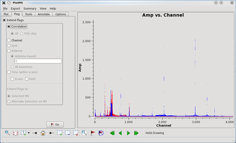
The plotms Flag tab. Here the Extend flags box has been checked, enabling the Correlation (selected) and Channel options. The plot shows unflagged data in blue and flagged data in red.
See the section below on interactive flagging in plotms. The options in this tab allows the user to have flagging extend to other data points besides what is marked on the plot.
When enabled with the Extend flags checkbox, the user may choose to extend flags based on correlation or channel by checking the corresponding checkboxes. Future options for flag extensions are planned.
By checking the boxes next to Extend Flags and Correlation, flags will be extended beyond the correlations displayed. Currently the only option is to extend to All correlations as noted by the radio button, implying that all correlations will be flagged. For example, with RR displayed, the correlations RR, RL, LR, and LL will all be flagged when this option is enabled.
By checking the boxes next to Extend Flags and Channel, flagging will be extended to other channels in the same spw as the displayed point. For example, if spw=’0:0’ and channel 0 is displayed, then flagging will extend to all channels in spw 0.
The plotms task parameter used to extend flags is extendflag (True/False, default is False) with subparameters extcorr (True/False), and extchannel (True/False). These parameters will enable flag extensions when interactively flagging the plot.
Interactive Tools: The Tools Tab, Annotate Tab, and Tool Icons
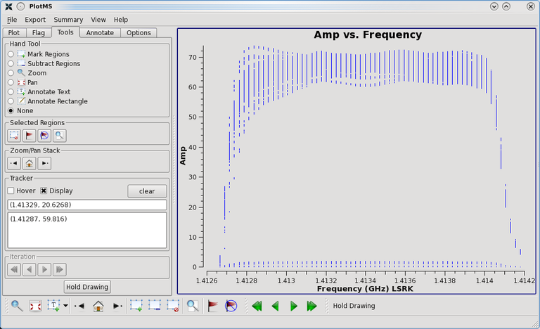
The plotms Tools tab. Here the Tracker Display tool is showing the (X,Y) coordinates of the cursor position. A previous position was saved to the text box by pressing the SPACE bar.
Various interactive GUI tools are selectable with the radio buttons in the Hand Tools section of the Tools tab at the top of the plotms window. They are also available as icon buttons at the bottom of the plotms window. These tools can be used to zoom, pan, annotate, flag/unflag, and locate data. Described below are the bottom icon buttons in order.

Zoom — The “magnifying glass” button (1st on left) lets you draw a box around a region of the plot (left-click on one corner of the box, and drag the mouse to the opposite corner of the desired box), and then zooms in on this box.
Pan — The “four-arrow” button (2nd from left) lets you pan around a zoomed plot.
Annotate — The 3rd button from the left is chosen from a drop-down menu to either Annotate Text (“T with a green diamond” button) or Annotate Rectangle (“pencil” button). With Annotate Text activated, click on a location in the plot where text is desired; a window will pop up, allowing you to type text in it. When you click the OK button, this text will appear on the plot. Annotate Rectangle simply lets you draw a box on the plot by left-clicking and dragging the mouse. By clicking on the Annotate tab near the top of the plotms window, different fonts, colors, line styles, etc. can be selected for annotations.
Stack Base — The “house” button (5th from left) returns to the original zoom level.
Stack Back and Stack Forward — The left and right arrow buttons (4th and 6th from left) step through the zoom settings you’ve visited.
Mark Regions — The “box with a green diamond” button (7th from left) lets you mark a region for flagging, unflagging, or locating. Left-click on one corner of the desired region, and then drag the mouse to set the opposite corner of the region. You can mark multiple boxes before performing an operation on them. The selected regions will appear on the plot as shaded rectangles.
Subtract Regions — The “box with a minus sign” button (8th from left) lets you de-select marked regions (draw around a marked region and the shaded area will disappear). To de-select all marked regions, use the next button.
Clear Regions — Clicking on the “box with a red circle” button (9th from left) will clear all regions which have been marked using Mark Regions.
Locate — The “magnifying glass on a sheet of paper” button (10th from left) will print out information about points in the marked regions. This information is printed to the shell terminal when plotms was started with casaplotms, or to the casa logger/logfile when plotms was started in a casa python session. The header of the output indicates the plotted X and Y axes and the range of values in the selected region. The output for each point includes scan, field, time, baseline, spw, channel, frequency, correlation, X, Y, and observation ID. By copying this list to a text file, or setting a new logfile with casalog.setlogfile as described in the CASA logger documentation, the Locate information can be edited to provide input for flagdata. To list an entire column, e.g. all visibilities for a source, use the listvis task or the table tools.
Flag — Click on the “flag” button (11th from left) to flag all points in the marked regions. See the section below on Interactive Flagging.
Unflag — Click on the “crossed-out flag” button (12th from left) to unflag any flagged points in the marked regions (even if not displayed).
Flag All — Click on the “per-grid flag/unflag” button (13th from left) to enter/leave the “Flag All” mode. See the section below on Interactive Flagging.
Iteration — The next four green arrow buttons (14th through 17th from left) control iteration, with the first and last “double arrow” buttons used to display the first and last iteration, and the center two “single arrow” button to display the previous or next iteration. If the plots are on a grid, these arrows navigate through the pages of plots which contain multiple iterations.
Hold Drawing — If the Hold Drawing button (rightmost, or 18th from left) is clicked to activate it, when new plot axes are selected from the Plot > Axes tab, the new data will be cached but not plotted. When the button is clicked again (de-activated), it will automatically plot the data that was last requested. This can be particularly useful when changing the size of the plotms window.
The Tools tab also contains Tracker tools including Hover and Display. When Hover is selected and the mouse is moved over the plot, the pointer’s position is displayed on the plot in (X, Y) format. When Display is selected, the (X, Y) position is displayed in the text box under the Display checkbox.
To record various tracked positions, enable Display then click on the plot to activate it. As usual, moving the pointer displays the position in the small display text box. Pressing the SPACE bar will copy the displayed line into the larger white box below it. This can be repeated many times and a log of positions and values will be created. The content in the box can then be easily copied and pasted into any other application that is used for data analysis. The Clear button wipes out the content of the box for a fresh start into new scientific adventures.
Miscellaneous Options: The Options Tab
A few miscellaneous per-page plot options and GUI options are available in the Options tab, the last tab at the top of the plotms window.
Plotting on a Grid
The layout of the page is set on the plotms Options tab. For multiple plots per page, set the grid layout, the number of rows and columns that determine the number of sub-plots. When set, click “Update” to activate the grid changes.
Plotting Iterations on a Grid
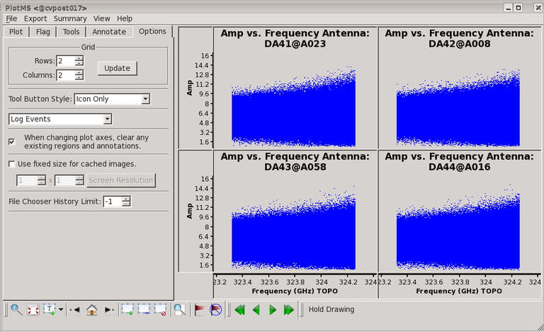
The plotms Options tab. Here a 2x2 grid has been created with iteration on the ‘antenna’ axis.
If iteration is enabled in the Plot > Page tab, the grid will be filled automatically with each iterated plot. The Plot > Page tab is also where common axis scales and shared axes will be set; they are enabled for the plot in Figure 9. These axis options are only available for iterated plots in a grid.
The plotms task parameters used to create a grid with iteration include gridrows and gridcols (default is 1). To create the plot shown in Figure 9, the plotms command would be:
plotms('ngc5921_ut.ms', xaxis='freq', iteraxis='antenna', gridrows=2, gridcols=2,
       xsharedaxis=True, xselfscale=True, ysharedaxis=True, yselfscale=True)
Plotting Multiple Data on a Grid
We note here that plotting multiple datasets or axes on a grid is possible in plotms but covered separately in the Plotting Multiple Data section below, as this involves many settings in the GUI or multiple plotms task commands. Since the grid affects all of the plots, its settings are in the Options tab rather than the Plot tab.
Tool Button Style
The Tool Button Style drop-down menu determines the format of the tool buttons at the bottom of the plotms window. The options include Icon Only, Text Only, Text Beside Icon, and Text Under Icon. In Icon Only mode (default), hovering the cursor over each icon will give a text description of the icon.
To hide the bottom icons, see the description of the View menu. The tools can also be accessed in the Tools tab.
Log Events
This drop-down menu shows a checklist of events and plotms functions so that you can customize how verbose plotms is in documenting its actions.
Clear Regions and Annotations
The When changing plot axes, clear any existing regions or annotations checkbox determines when regions and annotation are deleted from the plot. By default, this is enabled.
Cached Images
A useful option is the Use fixed size for cached image checkbox. It determines how large the dots in the panel are with respect to the screen resolution. The values influence how the data is redrawn on the panel. When Screen resolution is selected, the plotms window can be resized without redrawing on the canvas – a considerable speedup for large data sets. The penalty is that the dots of the data points are the size of a pixel on the screen, which may be very small for high resolution monitors. By default, this feature is not enabled.
File Chooser History Limit
This setting allows the user to limit how many remembered filepaths are displayed in file chooser dialogs produced by clicking Browse in the Plot > Data tab to select a MeasurementSet or calibration table and in the Plot > Calibration tab to select a calibration library.
The Plotms Menus
File Menu: Quit
The File menu in the top menu bar allows you to Quit plotms, or you can click the X in the upper right corner of the window.
Export Menu: Saving Your Plot
You can save a copy of a plot to file with the Export menu, which produces an Export Plots dialog box with many settings.
Filename: Click the Browse button for a GUI-based selection of the directory and filename to which the plot will be saved, or click the Insert MS Name button to minimize typing. You may also just type in a file name. The file format can be determined in this GUI by the suffix given to the filename: .png, .jpg, .ps, .pdf, and txt.
If a file already exists with the given filename, it will be overwritten without warning!
Format: Alternatively, the file format can be selected from the Format drop-down menu, with these options: [by file extension], PNG, JPG, PS, PDF, and TEXT. For the first option, if your filename is “test.jpg” the plot will be exported in JPG format. For the other formats, plotms will use the filename as given and not add a suffix to indicate its format. See below for an example of TEXT format; the header will include the name of the visibility and other specified parameters including selection, averaging, transformations, etc.
Verbose: When a text export is selected, the output can be verbose (include metadata). When this checkbox is unchecked, the text export will include x and y values only. This parameter is ignored for other formats.
Range: When iteration is chosen, producing multiple plots, you may select to export only the Current Page or All Pages. Each saved plot will have the name of the iteration appended to the given filename before the extension. For example, with filename “ngc5921_ut.jpg” and iteration on antenna, the first plot will be named ngc5921_ut_Antenna1@VLA:N7.jpg. This is so the exported plots can be identified without viewing them. Be warned that if you are plotting iterations on a grid, the filenames will have all of the iterations on the page appended, which can lead to a very long filename. Filenames exceeding 255 characters in length will be automatically shortened upon export. One plotfile per page is produced; multipage pdf exports are not currently supported.
High Resolution: Exporting to images in screen resolution is currently not working, so plot exports are always high resolution. A notice is issued in the console/log.
DPI, Size: Use the text boxes or up/down arrows to set the output DPI or size (in pixels) of the exported plot.
Export: When settings are complete, click Export to create your plotfile.
Note: The plot files produced by the PS and PDF options can be large and time-consuming to export. The JPG is the smallest.
The TEXT format will not save an image but all of the data points themselves. This allows one to dump the current plot into a file that is used in other programs for further processing.
ALERT: The exported TEXT file can be quite large and take some time to create. Using averaging, selection, etc. is recommended to keep the file size manageable. If a region is marked as described in the Interactive Tools section, only those points are exported to the text file.
The reported data is the same as when using the Locate button in plotms, with the following format (when verbose=True):
#vis: ngc5921_ut.ms
#scan: 4
#channel average: 63
#time average: None
#From plot 0
#x y chan scan field ant1 ant2 ant1name ant2name time freq spw corr obs
#Time Amp None None None None None None None MJD(seconds) GHz None None None
4304483429.999 62.7219 0 4 1 1 1 2@VLA:W1 2@VLA:W1 4304483429.999 1.413332233 0 RR 0
4304483429.999 59.0717 0 4 1 1 1 2@VLA:W1 2@VLA:W1 4304483429.999 1.413332233 0 LL 0
4304483429.999 59.0252 0 4 1 27 27 28@VLA:W7 28@VLA:W7 4304483429.999 1.413332233 0 RR 0
4304483429.999 60.8603 0 4 1 27 27 28@VLA:W7 28@VLA:W7 4304483429.999 1.413332233 0 LL 0
4304483429.999 57.4048 0 4 1 7 7 8@VLA:W8 8@VLA:W8 4304483429.999 1.413332233 0 RR 0
etc.
where x and y are the two plotted axes and the other columns contain additional information such as the baselines and frequencies, with an additional line for units. The header for the file includes the name of the visibility and other parameters such as selection, averaging, etc.
The plotms task parameter used to export plots is plotfile. Unlike the Export Plots dialog box in the GUI, plotms will issue an error if this file exists unless overwrite=True. Its subparameters include:
expformat (‘jpg’, ‘png’, ‘pdf’, ‘ps’, ‘txt’) - select the format if no extension is included in the plotfile. If there is no plotfile extension and no expformat set, the plot will be exported as a PNG.
verbose (True/False, default is True) - include metadata in text export; ignored for other formats.
exprange (‘current’, ‘all’; defaults to ‘current’) for iterated plots
highres (True/False, default is False)
dpi - dots per inch
width (in pixels)
height (in pixels)
overwrite (True/False, default is False)
Summary Menu: Information About Your Dataset
Information about the MeasurementSet can be obtained from within plotms by clicking on the Summary menu in the top menu bar. If All is chosen from the pull-down menu next to Type, listobs-style output about scans, correlator configurations, and antennae will be written to the console or log. Other options for a subset of the data include Where, What, How, Main, Tables, Antenna, Feed, Field, Observation, History, Polarization, Source, Spectral Window, Spectral Window and Polarization, SysCal, and Weather.
For calibration tables, options in the Summary menu include All, Where, What, How, Main, Tables, Antenna, Field, Observation, History, and Spectral Window.
For more detail, click on the Verbose checkbox.
View Menu: Hide or Display Tool Icons
This menu controls the display of tool icons. Use the View > Toolbars menu to de-select and hide the Tools, Iteration (green arrows), or Display (Hold Drawing) icons. By default these icons are all selected and displayed at the bottom of the plotms window.
Help Menu: About plotms
This menu’s About option describes plotms and the versions of CASA, Qt, and Qwt it uses, along with links. Qt is the software framework that plotms uses for its GUI, and Qwt is a library that provides plotting functionality on top of the Qt framework.
Click About Qt for more detail about this software package and its licensing.
Plotting Multiple Data
Overplotting Multiple Datasets or Axes on the Same Plot
It is possible to overplot two datasets on the same plot, or the same dataset with different y-axes in each plot. To do this, set up the first plot as usual. Then press the Add Plot button at the bottom left of the plotms window. This will bring up an additional data input panel in the Plot > Data tab where you can specify the plot parameters as you did for the first one, which is automatically minimized. Use the slider to scroll vertically through the panels. Use right-click options or the Minimize, Maximize, or Close buttons to keep a better overview on the individual datasets.
When overplotting, you may want to set different custom colors for each dataset in its Display tab. If you are plotting different axes or the axes ranges are a significantly different range of values, you may want to set different axes locations for each plot in the Axes tab. When you are done, click the Plot button to see the overplot.
Use the Close button in each data panel to close the panel and remove that plot.
In the plotms task interface, you can overplot by invoking plotms more than once with clearplots=False. Each plotms command corresponds to a plot to go on top of previous ones, and each must have its own plotindex (0-based, default is 0). Otherwise, with the same plotindex, the second plot will overwrite the first. In the following example, we are plotting Scan vs. Time for MeasurementSet test1.ms with plotindex 0, and Field vs. Time for MeasurementSet test2.ms on the same plot with plotindex 1. The test2 data is a different color and its yaxis is on the right.
Note that since the plotindex is an index into subplots, this parameter must be assigned in consecutive order. If a plotindex is skipped, plotms will adjust the index number and inform the user of the corrected plotindex value.
plotms(vis='test1.ms', yaxis='scan')
plotms(vis='test2.ms', yaxis='field', plotindex=1, clearplots=False, customsymbol=True, symbolcolor='00FF00', yaxislocation='right')
Plotting Multiple Datasets or Axes on a Grid
plotms allows you to plot more than one dataset or axes on the same page by specifying a grid size then a grid location for each plot as described below. Here is an example of two plots with different datasets:
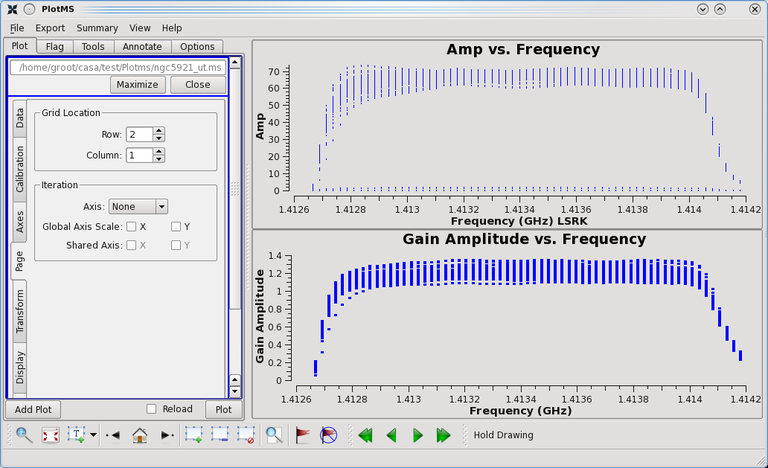
Plotting multiple data sets on a 2x1 grid. Here, the MS is plotted in grid location (1,1). Then the Add Plot button was used to select its bandpass calibration table and plot it in grid location (2,1).
The process is similar to the one above, except that you specify the grid and each plot’s location:
Set up your first plot as described above.
Use the Options tab to set up a grid by incrementing the number of rows and/or columns. By default the plot you set up in step 1 will be in row 0, column 0.
Use the Add Plot button to set up the second plot’s parameters. Pay particular attention to the new dataset’s Page tab, where you can set the Grid Location (row and column number) of the new plot. This section appears only when a grid is set up.
Unlike iteration, you cannot share axes among the plots.
Add as many plots as you desire to fill your grid, then click Plot.
Several plotms task parameters are used to create a grid and specify a plot location.
gridcols and gridrows define the number of plots on the screen.
colindex and rowindex (0-based) set the location of an individual plot
plotindex (0-based) must be incremented by 1 for each plotms call
clearplots is set to False to keep previous plots
Here is an example of multiple plotms calls to set up two plots on a grid and export the plot page; note the defaults on the first call are rowindex=0, colindex=0, plotindex=0 so just set up the grid. On each subsequent plotms call set clearplots=False and increment the plotindex by 1. To save the gridded plot, set a plotfile on the final plot.
plotms(vis='test1.ms', yaxis='field', gridrows=2, gridcols=1)
plotms(vis='test2.ms', yaxis='field', gridrows=2, gridcols=1, rowindex=1, colindex=0, plotindex=1, clearplots=False, plotfile='fields.jpg')
Interactive Flagging
Interactive flagging, on the principle of “see it — flag it”, is possible on the X-Y display of the data plotted by plotms. Mark one or more regions as described below, then flag or unflag the data that falls in these regions of the display.
Do not attempt to flag data while another task is accessing the same data set.
A note about Table locks
For plotting, plotms opens the MeasurementSet read-only, so there should be no problem if another task accesses the same dataset, unless the other task locks the file. When this happens, you can wait for the lock to be released, cancel cache-loading in the plotms dialog box, type go clearstat at the prompt, or exit plotms. Do not attempt to flag data in plotms while another task is accessing the same data set, as in this case plotms must open the MeasurementSet with a file lock for writing.
Mark data for flagging
Using the row of icons at the bottom of the plotms window, click on the Mark Regions button, then mark a region by left-clicking and dragging the mouse. Each click and drag will mark an additional region. You can remove all of your marked regions by clicking on the Clear Regions button. Once regions are marked, you can then click on one of the other buttons to take action:
Flag — flag all of the points in the region(s),
Unflag — unflag flagged points in the region(s),
Locate — list information (X and Y value, scan, field, baseline, frequency, etc.) about the points in the region(s) to the command line or log (Warning: this could be a long list!).
WARNING: If you Flag a region, using Unflag will not return the data to its previous state but will unflag all of the data in the marked region.
The following figure shows an example of marking regions and then clicking the Flag button. Whenever you click on a button, that action occurs without requiring an explicit disk-write. If you quit plotms and re-enter, you will see your previous edits because your flag changes were written to the MeasurementSet on disk.
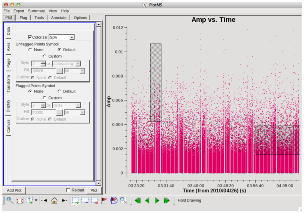
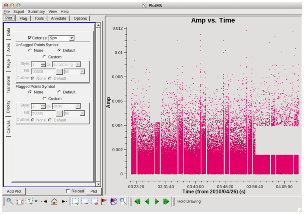
Plot of amplitude versus time, before (top) and after (bottom) flagging two marked regions. Note that flagged data is not displayed so these regions are not plotted after flagging. To unflag these regions, mark the two same regions and click the Unflag button.
New interactive flagging is available in CASA 5.5 and later. The button Flag All, which is located next to the Unflag button, can turn on and off “Flag all/Unflag all” mode by clicking it. Instead of flag/unflag operation on selected region, the “Flag all/Unflag all” mode allows you to flag/unflag whole data associated with the grid. The usage of this mode is as follows:
- Press the Flag All button – enter the “Flag all/Unflag all” mode. Background color of completely flagged grids will become yellow.
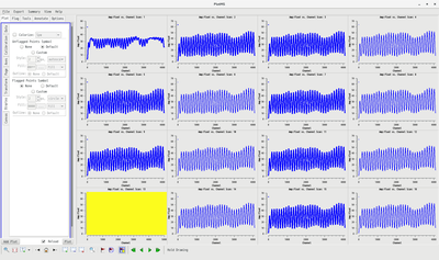
- Select grids to flag/unflag – click each grid to select for flag/unflag when the mode is active. Unflag is selected for the grids where all data are already flagged, otherwise flag is selected. The background color of the grids selected for flag will change to yellow while the grids selected for unflag will change to the default color.
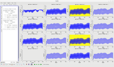
- Press the Flag All button again – leave the “Flag all/Unflag all” mode. At this moment, flag/unflag operations are applied to the data of the currently displayed grids selected in the previous step, and each grid is updated accordingly.
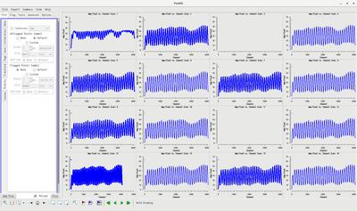
WARNING: On macOS, the “Flag all/Unflag all” mode does not work as expected!
On macOS, background color of grids doesn’t yet change properly although flag/unflag operations work fine. It is not recommended to use this mode on macOS.
WARNING: You cannot “undo” flagging to a previous state!
plotms does not automatically create flag backups in the <msname>.flagversions file. It is thus recommended to save the initial flags with the flagmanager task before starting plotms interactive flagging. Important intermediate flagging stages may also be saved during plotms flagging in the same fashion. Flagging can also be performed using the interactive msview task or scripted with the flagdata or flagcmd tasks.
WARNING: Use of flag extensions may lead to deletion of much more data than desired. Be careful!
Flags can also be extended with options in the Flag tab; see that section for a more detailed description of these options. Flag extension enables the user to plot a subset of the data and extend the flagging to a wider set. In this release, the only functional extensions are correlation and channel.
WARNING: Interactive flagging doesn’t support a collaboration with Iteration buttons!
The flag/unflag operations are applied to currently displayed grids only, although you can move to other iterations in the “Flag all/Unflag all” mode.
Scripting With No GUI
When scripting to produce exported plotfiles, set the plotms parameter showgui=False to suppress the GUI and pop-up dialog boxes which require a user response. The default is showgui=True.
Exiting plotms
To exit the plotms GUI, select Quit from the File menu at the top of the plotms window, or click the “X” on the frame.
Alternatively, plotms will keep running in the background and update with each subsequent plotms call. If the data file changes in the background while you are using other tasks, you can force reloading the data via the Reload checkbox next to the Plot button, or press SHIFT while clicking on Plot for the same purpose.
If started in a casa session, plotms will automatically quit when the session is ended.
Flag using flagdata
Flagging MeasurementSets and calibration tables
flagdata is the main flagging task in CASA. flagdata can flag MeasurementSets and calibration tables with an elaborate selection syntax. It also contains auto-flagging routines.
Other tasks related to flagging are flagmanager to save the existing flags before adding more, and plotms and msview for interactive flagging. In addition, optionally, data for which calibration solutions have failed will be flagged when these solutions are applied.
The inputs to flagdata are:
#In CASA
CASA<1>: inp flagdata
#flagdata :: All-purpose flagging task based on data-selections and flagging modes/algorithms.
vis              = ''          #Name of MS file or calibration table to flag
mode             = 'manual'    #Flagging mode
     field       = ''          #Field names or field index numbers: '' ==> all, field='0~2,3C286'
     spw         = ''          #Spectral-window/frequency/channel: '' ==> all, spw='0:17~19'
     antenna     = ''          #Antenna/baselines: '' ==> all, antenna ='3,VA04'
     timerange   = ''          #Time range: '' ==> all,timerange='09:14:0~09:54:0'
     correlation = ''          #Correlation: '' ==> all, correlation='XX,YY'
     scan        = ''          #Scan numbers: '' ==> all
     intent      = ''          #Observation intent: '' ==> all, intent='CAL*POINT*'
     array       = ''          #(Sub)array numbers: '' ==> all
     uvrange     = ''          #UV range: '' ==> all; uvrange ='0~100klambda', default units=meters
     observation = ''          #Observation ID: '' ==> all
     feed        = ''          #Multi-feed numbers: Not yet implemented
     autocorr    = False       #Flag auto-correlations

action           = 'apply'     #Action to perform in MS and/or in inpfile (none/apply/calculate)
     display     = ''          #Display data and/or end-of-MS reports at runtime (data/report/both).
     flagbackup  = True        #Back up the state of flags before the run

savepars         = False       #Save the current parameters to the FLAG_CMD table or to a file
vis can take a MeasurementSet or calibration table. Data selection for calibration tables is limited to field, scan, time, antenna, spw, and observation. See section at end about which parameters are applicable for calibration tables. Since calibration tables do not have a FLAG_CMD table, parameter settings, if requested, can only be saved in external files.
The *mode* parameter
The mode parameter selects the flagging algorithm and the following are available:
list        = list of flagging commands to apply to MS
manual      = flagging based on specific selection parameters
clip        = clip data according to values
quack       = remove/keep specific time range at scan beginning/end
shadow      = remove antenna-shadowed data
elevation   = remove data below/above given elevations
tfcrop      = automatic identification of outliers on the time-freq plane
rflag       = automatic detection of outliers based on sliding-window RMS filters
antint      = flag integrations if all baselines to a specified antenna are flagged
extend      = extend and/or grow flags beyond what the basic algorithms detect
summary     = report the amount of flagged data
unflag      = unflag the specified data
these are described in detail lower down.
Flagging will only be applied to the data selection that is performed with the usual selection parameters. The dataset is iterated-through in chunks (small pieces of data) consisting of one field, one spw, and a user-defined timerange (default is one scan). In addition to the typical antenna, spw, timerange, etc. selections, we would like to point out some addition of the correlation syntax for modes clip, tfcrop, and rflag. One can combine correlation products with simple mathematical expressions
'ABS', 'ARG', 'RE', 'IM', 'NORM'
where ABS is the absolute value, RE, the real and IM the imaginary part. NORM and ARG refer to the amplitude and phase. This parameter is followed by the polarization products (using an underscore in between “_” )
'ALL', 'I', 'XX', 'YY', 'RR', 'LL', 'WVR'
‘WVR’ refers to the water vapour radiometer of ALMA data. Note that the operators ABS,ARG,RE, etc. are written only once as the first value. if more than one correlation is given, the operator will be applied to all of them. An example would be
correlation = 'RE_XX, XY'
which would select all real XX and XY polarization for flagging.
The *action* parameter
The parameter action controls whether the actual flagging commands will be applied or not and the options are the empty string “, ‘apply’ and ‘calculate’.
apply is likely the most popular one as it applies the flags to the MS:
#In CASA:
action = 'apply' #Action to perform in MS and/or in inpfile
#(none/apply/calculate)
display = '' #Display data and/or end-of-MS reports at runtime
#(data/report/both).
flagbackup = True #Back up the state of flags before the run
flagbackup specifies if a backup of the current flags should be saved in the “*.flagversions” file. display can be “, ‘data’, ‘report’, ‘both’ where the empty string ” will report no individual flagging statistics, whereas ‘data’ launches an interactive GUI to display data and flags for each chunk to browse through. The plots are time-frequency planes and both old and new flags are being overlaid for all correlations per baseline. In the GUI, one can step though all chunks for inspection and if the flagging is unsatisfactory, one can exit without applying the flags. If the flagging is acceptable, it is also possible to continue flagging without viewing all chunks (the number of chunks can be very large for typical JVLA and ALMA data sets. display=’report’ lists the flagging statistics at the end of the procedure on the screen and both starts the GUI and reports all statistics at the end.
action=’calculate’ calculates the flags but does not write them to the MS or calibration table. This is useful if one would like to inspect the computed flags in the GUI without a straight application:
action  = 'calculate' #Action to perform in MS and/or in inpfile (none/apply/calculate)
display = ''          #Display data and/or end-of-MS reports at runtime (data/report/both).
The empty string action=” will do nothing and is useful when the commands themselves shall only be written to the FLAG_CMD sub-table or to an external file using the savepars parameter to specify the filename.
savepars will save the flagging commands to a file that can be later used for input in flagdata via mode=’list’. It also shares the flagcmd syntax and can be used there. The file name is specified by outfile and, if empty, the FLAG_CMD table in the MS will be populated. A REASON can be given by the reason parameter which may be useful for bookkeeping as well as for unflagging data that are marked by specific REASON parameters. The overwrite parameter will control overwriting an existing file when saving the flag commands.
Flagging Modes
Manual Flag/Unflag
mode = 'manual' #Flagging mode (list/manual/clip/shadow/quack/el
#evation/tfcrop/rflag/extend/unflag/summary)
field = '' #Field names or field index numbers: '' ==> all,
#field='0~2,3C286'
spw = '' #Spectral-window/frequency/channel: '' ==> all,
#spw='0:17~19'
antenna = '' #Antenna/baselines: '' ==> all, antenna
#='3,VA04'
timerange = '' #Time range: '' ==>
#all,timerange='09:14:0~09:54:0'
correlation = '' #Correlation: '' ==> all, correlation='XX,YY'
scan = '' #Scan numbers: '' ==> all
intent = '' #Observation intent: '' ==> all,
#intent='CAL*POINT*'
array = '' #(Sub)array numbers: '' ==> all
uvrange = '' #UV range: '' ==> all; uvrange ='0~100klambda',
#default units=meters
observation = '' #Observation ID: '' ==> all
feed = '' #Multi-feed numbers: Not yet implemented
autocorr = False #Flag auto-correlations
The ‘manual’ mode is the most straight-forward of all modes. All visibilities that are selected by the various data selection parameters will be flagged or unflagged, depending on the action parameter. autocorr is a shorthand for antenna=’*&&&’ to flag all auto correlations in the data.
List
mode = 'list' #Flagging mode (list/manual/clip/shadow/quack/el
#evation/tfcrop/rflag/extend/unflag/summary)
inpfile = '' #Input ASCII file, list of
#files or Python list of strings with

#flag commands.
reason = 'any' #Select by REASON types
A list of flag commands can be provided through a file or a list of files, specified by the inpfile parameter. Each input line may contain a flagging mode with data selection parameters as well as parameters that are specific to that mode. All parameters that are not set will be reset to their default values (default mode is ‘manual’). Each line of this file or list of strings will be taken as a command to the flagdata task. This mode=’list’ is similar to the task flagcmd with the inpmode=’list’ option.
An example for such a file would be:
mode='shadow'
mode='clip' clipminmax=[0,5] correlation='ABS_ALL'
mode='quack' quackmode='end' quackinterval=1.0
antenna='ea01' timerange='00:00:00~01:00:00'
antenna='ea11' timerange='00:00:00~03:00:00' spw='0~4'
Alternatively, this can be issued in the task directly like:
#In CASA:
CASA<1>: flagdata(vis='vis',mode='list',
inpfile=["mode='shadow'",
"mode='clip' clipminmax=[0,5] correlation='ABS_ALL'",
"mode='quack' quackmode='end' quackinterval=1.0"'
"antenna='ea01' timerange='00:00:00~01:00:00'",
"antenna='ea11' timerange='00:00:00~03:00:00' spw='0~4'"])
or via a variable
#In CASA:
CASA<1>:cmds=["mode='shadow',
"mode='clip' clipminmax=[0,5] correlation='ABS_ALL'",
"mode='quack' quackmode='end' quackinterval=1.0",
"antenna='ea01' timerange='00:00:00~01:00:00'",
"antenna='ea11' timerange='00:00:00~03:00:00' spw='0~4'"]

CASA<2>: flagdata(vis='vis',mode='list', inpfile=cmds)
The syntax needs to be written with quotes e.g. mode=’manual’ antenna=’ea10’. There should be no space between key=value. Spaces are used to separate pairs of parameters, not commas.
Clip
mode = 'clip' #Flagging mode (list/manual/clip/shadow/quack/
#elevation/tfcrop/rflag/extend/unflag/summary)
...
datacolumn = 'DATA' #Data column on which to operate
#(data,corrected,model,residual)
clipminmax = [] #Range to use for clipping
clipoutside = True #Clip outside the range, or within it
channelavg = False #Average over channels (scalar average)
timeavg = False #Average over time ranges
timebin = '' #Bin width for time averaging.
clipzeros = False #Clip zero-value data
in addition to the regular selection parameters, mode=’clip’ also has an option to select between a number of scratch columns in datacolumn. This includes the usual DATA, CORRECTED, etc., and also clipping based on data weights WEIGHT, WEIGHT_SPECTRUM as well as other MS columns. clipminmax selects the range of values to be clipped – usually this is combined with clipoutside=True to clip everything but the values covered in clipminmax. The data can also be averaged over the selected spw channel ranges by setting channelavg=True, or time averages via timeavg=True and setting of timebin. clip will also flag ‘NaN’, ‘inf’, and ‘-inf’ values by default and can flag exact zero values (these are sometimes produced by the JVLA correlator) using the clipzeros parameter.
Note : For modes clip, tfcrop and rflag, channel-ranges can be excluded from flagging by selecting ranges such as spw=’0:05;1063’. This is a way to protect known spectral-lines from being flagged by the autoflag algorithms.
Shadow
mode = 'shadow' #Flagging mode (list/manual/clip/shadow/quack/
#elevation/tfcrop/rflag/extend/unflag/summary)
...
tolerance = 0.0 #Amount of shadow allowed (in meters)
addantenna = '' #File name or dictionary with additional antenna names,
#positions and diameters
This option flags shadowed antennas, i.e. when one antenna blocks part of the aperture of a second antenna that is behind the first one. Shadowing can be gradual and the criterion for a shadow flag is when a baseline is shorter than radius1 + radius2 − tolerance (where the radii of the antennae are taken from the MS antenna subtable); see the figure below. addantenna may be used to account for shadowing when antennas are not listed in the MS but are physically present. Please read the flagdata inline help for the syntax of this option.
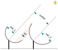
This figure shows the geometry used to compute shadowed antennas.
Quack
mode = 'quack' #Flagging mode (list/manual/clip/shadow/quack/
#elevation/tfcrop/rflag/extend/unflag/summary)
...
quackinterval = 0.0 #Quack n seconds from scan beginning or end
quackmode = 'beg' #flag an interval at the beginning of scan
'endb' #flag an interval at the end of scan
'tail' #flag all but an interval at the beginning of
scan
'end' #flag all but an interval at end of scan

quackincrement = False #Flag incrementally in time?
quack is used to remove data at scan boundaries. quackinterval specifies the time in seconds to be flagged, and quackmode can be ‘beg’ to flag the quackinterval at the beginning of each selected scan, ‘endb’ at the end of scan. ‘tail’ flags all but the beginning of scan and ‘end’ all but the end of scan. The quackincrement is either True or False, depending if one wishes to flag the quackinterval from the first unflagged data in the scan, or from the scan boundaries independent of data being already flagged or not.
Because quackincrement=True needs to know the state of the previous flags in order to know which is the first unflagged data, it cannot be used in ‘list’ mode, unless it is the first command of the list.
Visual representation of quack mode when flagging a scan
with 1s duration. The following diagram shows what is flagged
for each quack mode when quackinterval is set to 0.25s.
The flagged part is represented by crosses (+++++++++)

scan with 1s duration

--------------------------------------------
beg
+++++++++++---------------------------------
endb
---------------------------------+++++++++++
tail
-----------+++++++++++++++++++++++++++++++++
end
+++++++++++++++++++++++++++++++++-----------
Elevation
mode = 'elevation' #Flagging mode (list/manual/clip/shadow/quack/
#elevation/tfcrop/rflag/extend/unflag/summary)
...
lowerlimit = 0.0 #Lower limiting elevation (in degrees)
upperlimit = 90.0 #Upper limiting elevation (in degrees)
Flagging based on the elevation of the antennae. This may be useful to avoid data taken at very low elevations or close to transit and the lowerlimit and upperlimit parameters specify the range of good elevations.
Tfcrop
mode = 'tfcrop' #Flagging mode (list/manual/clip/shadow/quack/
#elevation/tfcrop/rflag/extend/unflag/summary
#)
...
ntime = 'scan' #Time-range to use for each chunk (in seconds
#or minutes)
combinescans = False #Accumulate data across scans.
datacolumn = 'DATA' #Data column on which to operate
#(data,corrected,model,residual)
timecutoff = 4.0 #Flagging thresholds in units of deviation
#from the fit
freqcutoff = 3.0 #Flagging thresholds in units of deviation
#from the fit
timefit = 'line' #Fitting function for the time direction
#(poly/line)
freqfit = 'poly' #Fitting function for the frequency direction
#(poly/line)
maxnpieces = 7 #Number of pieces in the polynomial-fits (for
#'freqfit' or 'timefit' = 'poly')
flagdimension = 'freqtime' #Dimensions along which to calculate fits
#(freq/time/freqtime/timefreq)
usewindowstats = 'none' #Calculate additional flags using sliding
#window statistics (none,sum,std,both)
halfwin = 1 #Half-width of sliding window to use with
#'usewindowstats' (1,2,3).
extendflags = True #Extend flags along time,
#frequency and correlation.
channelavg = False #Pre-average data across channels before
#analyzing visibilities for flagging.
chanbin = False #Bin width for channel average in
#number of input channels.
timeavg = False #Pre-average data across time before
#analyzing visibilities for flagging
timebin = False #Bin width for time average in seconds
TFCrop is an autoflag algorithm that detects outliers on the 2D time-frequency plane, and can operate on un-calibrated data (non bandpass-corrected). The original implementation of this algorithm is described in NCRA Technical Report 202 (Oct 2003).
The algorithm iterates through the data in chunks of time. For each chunk, the result of user-specified visibility-expressions are organized as 2D time-frequency planes, one for each baseline and correlation-expression result, and the following steps are performed.
As of CASA 4.6 the data can also be pre-averaged over the selected spw channel ranges by setting channelavg=True and chanbin to the desired bin (in number of channels), or time averaged over the selected time ranges by setting timeavg=True and timebin to the desired time range (in seconds). This averaging is independent from the tfcrop time/channel average, and allows to specify custom time/channel average bins, instead of averaging all data across time and/or channel direction.
Calculate a bandshape template : Average the data across time, to construct an average bandpass. Construct an estimate of a clean bandpass (without RFI) via a robust piece-wise polynomial fit to the average bandpass shape.
Note : A robust fit is computed in up to 5 iterations. It begins with a straight line fit across the full range, and gradually increases to ‘maxnpieces’ number of pieces with third-order polynomials in each piece. At each iteration, the stddev between the data and the fit is computed, values beyond N-stddev are flagged, and the fit and stddev are re-calculated with the remaining points. This stddev calculation is adaptive, and converges to a value that reflects only the data and no RFI. At each iteration, the same relative threshold is applied to detect flags, and this results in a varying set of flagging thresholds, that allows deep flagging only when the fit represents the true data best. Iterations stop when the stddev changes by less than 10%, or when 5 iterations are completed.
The resulting clean bandpass is a fit across the base of RFI spikes.
Divide out this clean bandpass function from all timesteps in the current chunk. Now, any data points that deviate from a mean of 1 can be considered RFI. This step helps to separate narrow-band RFI spikes from a smooth but varying bandpass, in situations where a simple range-based clipping will flag good sections of the bandpass.
Perform iterative flagging (robust flagging) of points deviating from a value of 1.
Flagging is done in up to 5 iterations. In each iteration, for every timestep, calculate the stddev of the bandpass-flattened data, flag all points further than N times stddev from the fit, and recalculate the stddev. At each iteration, the same relative threshold is applied to detect flags. Optionally, use sliding-window based statistics to calculate additional flags.
Repeat steps 1 and 3, but in the other direction (i.e. average the data across frequency, calculate a piece-wise polynomial fit to the average time-series, and find flags based on deviations w.r.to this fit.)
The default parameters of the tfcrop implementation are optimized for strong narrow-band RFI (see the example figure below). With broad-band RFI, the piece-wise polynomial can sometimes model it as part of the band-shape, and therefore not detect it as RFI. In this case, reducing the maximum number of pieces in the polynomial can help. This algorithm usually has trouble with noisy RFI that is also extended in time of frequency, and additional statistics-based flagging is recommended (via the ‘usewindowstats’ parameter). It is often required to set up parameters separately for each spectral-window.
If frequency ranges of known astronomical spectral lines are known a-priori , they can be protected from automatic flagging by de-selecting those frequency-ranges via the ‘spw’ data-selection parameter.
The extendflag parameter will clean up small portions of data between flagged data points along time and/or frequency when more than 50% of all timeranges or 80% of all channels are already flagged. It will also extend the flags to the other polarizations. Alternatively, mode=’extend’ can be used (see section below).
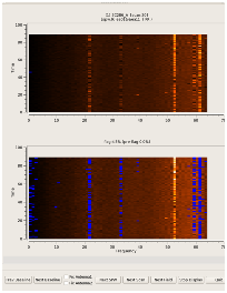
This screenshot represents a run where ‘tfcrop’ was run on a spw=’9’ with mainly narrow-band RFI. RIGHT : An example of protecting a spectral line (in this case, demonstrated on an RFI spike) by setting the spw-selection to spw=’0:0 45;53 63’. In both figures, the top row indicates the data before flagging, and the bottom row after flagging.
Rflag
mode = 'rflag' #Flagging mode (list/manual/clip/shadow/quack/
#elevation/tfcrop/rflag/extend/unflag/summary
#)
...
ntime = 'scan' #Time-range to use for each chunk (in seconds
#or minutes)
combinescans = False #Accumulate data across scans.
datacolumn = 'DATA' #Data column on which to operate
#(data,corrected,model,residual)
winsize = 3 #Number of timesteps in the sliding time
#window [aips:fparm(1)]
timedev = '' #Time-series noise estimate [aips:noise]
freqdev = '' #Spectral noise estimate [aips:scutoff]
timedevscale = 5.0 #Threshold scaling for timedev [aips:fparm(9)]
freqdevscale = 5.0 #Threshold scaling for freqdev
#[aips:fparm(10)]
spectralmax = 1000000.0 #Flag whole spectrum if freqdev is greater
#than spectralmax [aips:fparm(6)]
spectralmin = 0.0 #Flag whole spectrum if freqdev is less than
#spectralmin [aips:fparm(5)]
extendflags = True #Extend flags along time, frequency and correlation.
channelavg = False #Pre-average data across channels before
#analyzing visibilities for flagging.
chanbin = False #Bin width for channel average in
#number of input channels.
timeavg = False #Pre-average data across time before
#analyzing visibilities for flagging
timebin = False #Bin width for time average in seconds
RFlag is an autoflag algorithm based on a sliding window statistical filter. The RFlag algorithm was originally developed by Eric Greisen in AIPS (31DEC11). AIPS documentation : Subsection E.5 of the AIPS cookbook (Appendix E : Special Considerations for JVLA data calibration and imaging in AIPS http://www.aips.nrao.edu/cook.html#CEE)
In RFlag, the data is iterated-through in chunks of time, statistics are accumulated across time-chunks, thresholds are calculated at the end, and applied during a second pass through the dataset.
The CASA implementation also optionally allows a single-pass operation where statistics and thresholds are computed and also used for flagging, within each time-chunk (defined by ‘ntime’ and ‘combinescans’).
For each chunk, calculate local statistics, and apply flags based on user supplied (or auto-calculated) thresholds.
As of CASA 4.6 the data can also be pre-averaged over the selected spw channel ranges by setting channelavg=True and chanbin to the desired bin (in number of channels), or time averaged over the selected time ranges by setting timeavg=True and timebin to the desired time range (in seconds). This averaging is independent from the rflag time/channel sliding window, as it performs not only an average but also a binning operation (so there is no data overlap between adjacent bins), and allows to specify independent time/channel bins.
Time analysis (for each channel)
Calculate local rms of real and imag visibilities, within a sliding time window
Calculate the median rms across time windows, deviations of local rms from this median, and the median deviation
Flag if local rms is larger than timedevscale x (medianRMS + medianDev)
Spectral analysis (for each time)
Calculate avg of real and imag visibilities and their rms across channels
Calculate the deviation of each channel from this avg, and the median-deviation
Flag if deviation is larger than freqdevscale x medianDev
The extendflags parameter will clean up small portions of data between flagged data points along time and/or frequency when more than 50% of all timeranges or 80% of all channels are already flagged. It will also extend the flags to the other polarizations. Alternatively, mode=’extend’ can be used.
Some examples (see figure below):
Calculate thresholds automatically per scan, and use them to find flags. Specify scale-factor for time-analysis thresholds, use default for frequency.
#In CASA:
CASA<1>: flagdata('my.ms', mode='rflag',spw='9',timedevscale=4.0)
Supply noise-estimates to be used with default scale-factors.
#In CASA:
CASA<1>: flagdata(vis='my.ms', mode='rflag', spw='9', timedev=0.1, freqdev=0.5);
Two-passes. This replicates the usage pattern in AIPS.
The first pass saves commands in an output text files, with auto-calculated thresholds. Thresholds are returned from rflag only when action=’calculate’ (calc-only mode). The user can edit this file before doing the second pass, but the python-dictionary structure must be preserved.
The second pass applies these commands (action=’apply’).
#In CASA:
    CASA<1>: flagdata(vis='my.ms', mode='rflag', spw='9,10', timedev='tdevfile.txt', freqdev='fdevfile.txt', action='calculate');
    CASA<2>: flagdata(vis='my.ms', mode='rflag', spw='9,10', timedev='tdevfile.txt', freqdev='fdevfile.txt', action='apply');
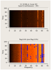
Example of rflag on narrow-band RFI
Extend
mode = 'extend' #Flagging mode (list/manual/clip/shadow/quack/el
#evation/tfcrop/rflag/extend/unflag/summary)
field = '' #Field names or field index numbers: '' ==> all,
#field='0~2,3C286'
spw = '' #Spectral-window/frequency/channel: '' ==> all,
#spw='0:17~19'
antenna = '' #Antenna/baselines: '' ==> all, antenna
#='3,VA04'
timerange = '' #Time range: '' ==>
#all,timerange='09:14:0~09:54:0'
correlation = '' #Correlation: '' ==> all, correlation='XX,YY'
scan = '' #Scan numbers: '' ==> all
intent = '' #Observation intent: '' ==> all,
#intent='CAL*POINT*'
array = '' #(Sub)array numbers: '' ==> all
uvrange = '' #UV range: '' ==> all; uvrange ='0~100klambda',
#default units=meters
observation = '' #Observation ID: '' ==> all
feed = '' #Multi-feed numbers: Not yet implemented
ntime = 'scan' #Time-range to use for each chunk (in seconds or
#minutes)
combinescans = False #Accumulate data across scans.
extendpols = True #If any correlation is flagged, flag all
#correlations
growtime = 50.0 #Flag all 'ntime' integrations if more than X%
#of the timerange is flagged (0-100)
growfreq = 50.0 #Flag all selected channels if more than X% of
#the frequency range is flagged(0-100)
growaround = False #Flag data based on surrounding flags
flagneartime = False #Flag one timestep before and after a flagged
#one (True/False)
flagnearfreq = False #Flag one channel before and after a flagged one
#(True/False)
Although the modes tfcrop and rflag already have extendflags parameters, some autoflagging algorithms may still leave small islands of unflagged data behind, data that are surrounded by flagged visibilities in the time-frequency space. Although the algorithm may deem these visibilities as good ones, they are frequently affected by low-level RFI that spills from the adjacent, flagged points and one may wish to clean those up.
ntime specifies the time ranges over which to clean up, e.g. ‘1.5min’ or ‘scan’ which checks on all data within a scan. To span time ranges larger than scans, one can set combinescans to True.
extendpols=True would extend all flags to all polarization products when at least one of them is flagged.
growtime flags the entire time range for a flagged channel, when a certain fraction of flagged time intervals is exceeded.
growfreq is similar but extends the flags in frequency when a given fraction of channels is already flagged.
growaround checks for flagged data points in the time-frequency domain that neighbor a datum. The threshold is four data points. If more surrounding points are flagged, the central datum will be flagged, too.
flagneartime flags adjacent data points along the time axis, around a flagged datum
flagnearfreq flags neighboring channels.

This screenshot represents a run where ‘tfcrop’ was run only on ‘ABS_RR’ (top row) and followed by an extension along time and correlations (bottom row).
Unflag
mode = 'unflag' #Flagging mode (list/manual/clip/shadow/quack/
#elevation/tfcrop/rflag/extend/unflag/summary
#)
field = '' #Field names or field index numbers: ''==>all,
#field='0~2,3C286'
spw = '' #spectral-window/frequency/channel
antenna = 'ea01' #antenna/baselines: ''==>all, antenna
#='3,VA04'
timerange = '' #time range:
#''==>all,timerange='09:14:0~09:54:0'
correlation = '' #Select data based on correlation
scan = '' #scan numbers: ''==>all
intent = '' #Select data based on observation intent:
#''==>all
feed = '' #multi-feed numbers: Not yet implemented
array = '' #(sub)array numbers: ''==>all
uvrange = '' #uv range: ''==>all; uvrange ='0~100klambda',
#default units=meters
observation = '' #Select data based on observation ID: ''==>all
The selection data will be unflagged.
Summary
mode = 'summary' #Flagging mode (list/manual/clip/shadow/quack/
#elevation/tfcrop/rflag/extend/unflag/summary
#)
...
minrel = 0.0 #minimum number of flags (relative)
maxrel = 1.0 #maximum number of flags (relative)
minabs = 0 #minimum number of flags (absolute)
maxabs = -1 #maximum number of flags (absolute). Use a
#negative value to indicate infinity.
spwchan = False #Print summary of channels per spw
spwcorr = False #Print summary of correlation per spw
basecnt = False #Print summary counts per baseline
This mode reports the number of rows and data points that are flagged. The selection of reported points can be restricted (see inline help for details).
mode=’summary’ can also report back a dictionary if the task is run as
#In CASA:
CASA<1>: s = flagdata(..., mode='summary')
with a variable assigned, here ‘s’.
Advanced: flagdata
Advanced Information on flagdata. C++ code infrastructure…
–CASA Developer–
For advanced information about some parts of flagdata please visit:
http://www.aoc.nrao.edu/~rurvashi/FlaggerDocs/FlaggerDocs.html
In progress…
C++ Infrastructure
Main Classes
AgentFlagger: The top-level AgentFlagger class that connects all of the following together, and defines the C++ user-interface for the agentflagger. This is the class used by the tool layer.
FlagDataHandler : A top level class defining the data handling interface for the flagging module.
FlagMSHandler: - TBD
FlagCalTableHandler: - TBD
FlagAgentBase: base class that defines the behaviour of all flagging agents and contains agent-level data-selection, etc. The main functions to be implemented by derived classes are setAgentParameters(), preProcessBuffer(), computeAntennaPairFlags() or computeRowFlags(), getReport() .
List of available Flag Agents :
1.  FlagAgentManual : Flag/Unflag based on data-selections. The only processing done by this agent is to set the flags for all data it sees to True if the operation is to flag, and to False to unflag. A boolean parameter apply determines whether to flag (apply=True) or unflag (apply=False). By default it is set to True.

2.  FlagAgentQuack : Flag time-ranges at the beginning and/or end of scans. Uses the YYY iteration-mode.

3.  FlagAgentElevation : Flag time-ranges based on source elevation. Uses the YYY iteration-mode.

4.  FlagAgentShadow : For each timestep, flag antennas that are shadowed by any other antenna. Antennas to be flagged are chosen and marked in the preProcess() stage. Rows are flagged in computeRow(), and this agent uses the YYY iteration-mode.

5.  FlagAgentExtension : Read and extend flags along specified axes, within the current chunk. Uses the YYY iteration-mode.

6.  FlagAgentClip : Flag based on a clip threshold and visExpression. Find and flag NaNs and Infs. Uses the YYY iteration-mode.

7.  FlagAgentTimeFreqCrop : The TFCrop algorithm is run per baseline, via FlagAgentTimeFreqCrop::computeAntennaPairFlags()

8.  FlagAgentRFlag : The RFlag algorithm. Implements multiple passes through each chunk via the passIntermediate() and passFinal() mechanism.

9.  FlagAgentSummary : Flag counts are accumulated in computeRow() and packaged into a Record in getResult().

10. FlagAgentDisplay : Visibilities are read and displayed from computeAntennaPair(). Navigation-buttons control the order in which the framework iterates through baselines.

11. FlagAgentAntennaIntegrations - TBD
The FlagReport class allows each flag agent to build and return information (summary counts, reports as plots, etc) to the user (and/or) to the display agent for end-of-MS reports.
Control Flow
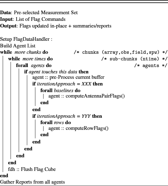
Performance and Optimizations
There are several performance-optimization choices that can be made. Some of these are under the users control, and some have automated heuristics.
List mode
It helps to combine multiple flag commands into a single run ONLY if most of the commands require the same data to be read. The goal is to read data once, apply multiple flag commands, and write flags once.
Manual-flag commands read only meta-data.
Shadow, elevation read meta-data + processing to calculate uvw, azel.
Clip reads visibilities.
tfcrop and rflag read visibilities and flags
Extend, summary read flags
Data Pre-selection
If only a subset of the Measurement Set is to be traversed for flag-calculation, it helps to pre-select and iterate through only that section of the MS. When flagdata is run in list mode, there is a second level of selection per agent (command) that ensures that each agent sees only its correct subset of the data.
Asynchronous I/O
Asynchronous I/O is a data-access optimization that applies when iterating through the dataset in chunks. It uses multi-threading to pre-read the next chunk of data from disk while the current chunk is being processed.
The user has the option of enabling asynchronous I/O by setting the following variables in the .casarc file.
VisibilityIterator.async.enabled: true     # if present and set to false then async i/o will work
VisibilityIterator.async.nBuffers: 2       # the default value is two
VisibilityIterator.async.logFile: stderr   # Send async i/o debug log messages to this file
                                           # if not present or file is invalid then no logging occurs
VisibilityIterator.async.logLevel: 2       # Level of log messages to output (two is good, too); defaults to 1

FlagDataHandler.asyncio: true              # True : enable async-IO for the flagger (clip,tfcrop,rflag)
FlagDataHandler.slurp: true                # True : enable ??
FlagAgent.background: true                 # True : enable threading mode
Asynchronous I/O helps only when data I/O dominates the total cost. For our current list of agents/algorithms, this helps only for agents that read visibilities. Therefore asynchronous I/O is activated only if clip or tfcrop or rflag are present in the flag-command list.
Flag using flagcmd
Flag the visibility data set or calibration table based on a specified list of flagging commands
Info: We recommend using task flagdata as the preferable and safer way for flagging based on the visitibilites inspection and for many other capabilities. The option to import XML files with online flag in flagcmd has largely become obsolete with the deprecation of importevla, because the recommended importasdm task cannot copy the actual XML tables from the original SDM to the newly created MS (it can only apply the online flags directly, or write them into ascii tables).
The task flagcmd will flag the visibility data set or calibration table based on a specified set of flagging commands using a flagging syntax. These commands can be input from the FLAG_CMD table within the MS, from an ascii file, or from input python strings. Input can also be from an XML table within a VLA SDM, but given that importasdm does not copy XML files (and importevla is deprecated), the Flag.xml, Antenna.xml and SpectralWindow.xml tables must first be copied manually into the top-level MS directory for use by flagcmd (not the recommended approach). Facilities for manipulation, listing, or plotting of these flags are also provided.
When doing any flagging with flagcmd it is wise to use the flagbackup=True parameter to save the current flags into a .flagversions file. See flagmanager for more details about this.
Alert: The FLAG_CMD sub-table is meant only for meta-data selections such as online flags. Using it to save other parameters (from modes such as clip, quack, shadow, etc) is possible but carries a risk that in future releases these parameters maybe renamed or changed their default values. There will be no automatic way to rename any parameter that changes in the future.
Alert: There is no way to guarantee that a command from the COMMAND column has been applied or not to the MS, even if the APPLIED column is set to True. If you use other ways to flag such as interactive flagging in plotms, the FLAG_CMD will not be updated! Use at your own risk!
The inputs to flagcmd are:
#flagcmd :: Flagging task based on batches of flag-commands
vis                 =      ''          #Name of MS file or calibration table to flag
inpmode             =      'table'     #Input mode for flag commands(table/list/xml)
inpfile             =      ''          #Source of flag commands
[tablerows           =      []          #Rows of inpfile to read]
reason              =      'any'       #Select by REASON types
useapplied          =      False       #Select commands whose rows
                                       #have APPLIED column set to True
action              =      'apply'     #Action to perform in MS and/or in inpfile
                                       #(apply/unapply/list/plot/clear/extract)
flagbackup          =      True        #Automatically backup the
                                       #FLAG column before execution
savepars            =      False       #Save flag commands to the MS or to a file
The default input mode is inpmode=’table’ which directs the task to input flag commands from the FLAG_CMD internal MS table. Other options include list and xml, explained below.
The default operation mode is action=’apply’ directing the task to apply relevant flagging commands to the MS data main table. Other options include ‘unapply’, ‘list’, ‘plot’, ‘clear’, and ‘extract’, explained below.
See the Flagging Command Syntax section below for more detail.
Alert: It is possible to flag calibration tables using flagcmd, although we recommend using the flagdata task for this in most cases.
When using flagcmd to flag calibration tables, only the apply and list actions are supported. Because calibration tables do not have a FLAG_CMD sub-table, the default inpmode=’table’ can only be used if an MS is given in the inpfile parameter so that flags from the MS are applied to the calibration table directly. Otherwise, the flag commands must be given using inpmode=’list’, either from a file or from a list of strings.
Input modes inpmode:
The inpmode parameter selects options for the input mode for the flagging commands.
Available inpmode options are:
‘table’ — input from MS table
‘list’ — input from ASCII file or from a list of strings
‘xml’ — input from XML table (largely obsolete with the deprecation of importevla in CASA 5.4)
The default input mode is inpmode=’table’ which directs the task to input flag commands from a FLAG_CMD MS table. This has the sub-parameters:
inpmode        =      'table'      #Input mode for flag commands(table/list/xml)
inpfile        =      ''           #Source of flag commands
[tablerows      =      []           #Rows of inpfile to read]
reason         =      'any'        #Select by REASON types
useapplied     =      False        #Select commands whose rows
                                   #have APPLIED column set to
                                   #True
If inpfile = ‘’ then it will look for the FLAG_CMD table in the MS given by vis. You can use this sub-parameter to tell the task to read the FLAG_CMD table from another MS and apply then to the MS given in vis.
The tablerows sub-parameter is a simple Python list of the row numbers of the table to consider in processing flags. The default is all rows. Currently it only takes fully-enumerated integer lists. Use the Python range function to generate ranges,
tablerows = range(0,30) + range(50,55)

#Do not use strings such as '0~29,50~54'
The useapplied sub-parameter toggles whether only flag commands marked as not having been applied are considered (the default), or to allow (re)processing using all commands.
The reason sub-parameter selects the reason type to process. The default ‘any’ means all commands.
Info: what is within the string is literally matched, e.g. reason=’’ matches only blank reasons, and reason = ‘FOCUS_ERROR,SUBREFLECTOR_ERROR’ matches this compound reason string only. To flag by either of these reasons alone, run flagcmd twice, once with reason=’FOCUS_ERROR’, and then with the other reason.
One use case is to read the flag commands from the FLAG_CMD of an MS and apply them to a calibration table given in the parameter vis. Example:
flagcmd(vis='cal-X54.B1', inpmode='table',inpfile='uid___A002_X2a5c2f_X54.ms', action='apply')
Input mode inpmode=’list’
See flagdata help for syntax.
This mode allows one to give a list of strings with flagging commands, the name of a file or a list of filenames that contains these commands equivalent to the mode=’list’ in flagdata. E.g. a file * flags.txt* that contains
scan='1~3' mode='manual'
mode='clip' clipminmax=[0,2] correlation='ABS_XX' clipoutside=False
spw='9' mode='tfcrop' correlation='ABS_YY' ntime=51.0
mode='extend' extendpols=True
can be used via
flagcmd(vis='some.ms',inpmode='list',inpfile='flags.txt')
A list of input files can also be given:
flagcmd(vis='some.ms',inpmode='list',inpfile=['flags.txt,'userflags.txt'])
Alternatively, the individual flagging commands can be directly provided in the call itself such as:
inpfile=["scan='1~3' mode='manual'",
        "mode='clip' clipminmax=[0,2] correlation='ABS_XX' clipoutside=False",
        "spw='9' mode='tfcrop' correlation='ABS_YY' ntime=51.0",
        "mode='extend' extendpols=True"]
Input mode inpmode=’xml’
Alert: With the deprecation of importevla, XML files can no longer be imported directly from the original SDM into the newly created MS, but only by manually copying the Flag.xml, Antenna.xml and SpectralWindow.xml tables into the top-level MS directory (not the recommended approach). Also, the XML mode is not available for cal tables, therefore it will not work for ALMA MSs. However, task importasdm with process_flags=True will copy the flags from the XML files directly to the FLAG_CMD sub-table, see importasdm help for options. This is the recommend way of dealing with the online flags.
The input mode inpmode=’xml’ tells the task to input flag commands from XML SDM files, which contain the online flags. When set this opens the sub-parameters:
inpmode        =      'xml'        #Input mode for flag commands(table/list/xml)
tbuff          =      0.0          #Time buffer (sec) to pad flags
ants           =      ''           #Allowed flag antenna names to select by
reason         =      'any'        #Select by REASON types
This mode will look for files called Flag.xml, Antenna.xml and optionally SpectralWindow.xml inside the MS directory specified under vis.
Info: You can only apply the flags from an XML file. It is not possible to unapply them. For that, transfer the flags to the FLAG_CMD table using action=’list’, then unapply them.
The tbuff sub-parameter sets a padding buffer (in seconds) to the begin and end times of the online flags in the XML file. The online flag time buffer tbuff is specified in seconds, but in fact should be keyed to the intrinsic online integration time to allow for events (like slewing) that occur within an integration period. This is particularly true for JVLA data, where a tbuff value of 0.5× to 1.5× the integration time is needed. For example, if data were taken with 1-second integrations, then at least tbuff=0.5 should be used, likewise tbuff=5 for 10-second integrations.
Info: For JVLA data you should use 1.5× (e.g. tbuff=15 for 10-second integrations) for data taken in early 2011 or before due to a timing error. We do not yet know what ALMA data will need for padding (if any).
The ants sub-parameter selects the antennas from which online flags will be selected (default is all antennas). For example, ants=’ea01’ is a valid choice for JVLA data.
The reason sub-parameter selects by the REASON field in the Flag.xml file. The default ‘any’ means all commands. Note that reason=” would only select flags who have a blank REASON field entry.
Operation types action
The action selects options for operating on the selected flags and possibly the data.
Available action options are:
‘apply’ — apply flag commands to data
‘unapply’ — unapply flags in data
‘list’ — list and/or save flag commands
‘plot’ — plot flag commands
‘clear’ — clear rows from FLAG_CMD table
‘extract’ — extract internal flag dictionary
Apply flags action=’apply’
The default operation mode is action=’apply’ directing the task to apply relevant flagging commands to the vis data main table.
action         =       'apply'     #Action to perform in MS and/or in inpfile
                                   #(apply/unapply/list/plot/clear/extract)
flagbackup     =       True        #Automatically backup the
                                        #FLAG column before execution
The flagbackup parameter toggles whether a new copy of the MS FLAG column is written to the .flagversions backup directory for that MS before the requested flagging operation.
Unapply flags action=’unapply’
The unapply option allows unflagging of data based on the selected flag commands. This choice opens the sub-parameters:
action = 'unapply' #Action to perform in MS and/or in inpfile
 #(apply/unapply/list/plot/clear/extract)
 flagbackup = True #Automatically backup the
 #FLAG column before execution
As in action=’apply’, it is possible to make a backup to the *.flagversions file by using flagbackup=True.
List and save flags action=’list’
The ‘list’ option will give a listing of the flagging commands. This choice opens the sub-parameters:
action = 'list' #Action to perform in MS and/or in inpfile
 #(apply/unapply/list/plot/clear/extract)
 savepars = True #Save flag commands to the MS or to a file
 outfile = '' #Name of output file to save commands
 overwrite = True #Overwrite an existing file to save the flag commands
This action lists the commands on the screen without applying them. One can save the flagging script to an file specified in the outfile parameter when savepars=True. If outfile is empty, it will save the commands to a new row in the MS FLAG_CMD table given in vis.
The format of the listing output depends on the source of the flagging commands. A set of flagging commands specified through inpmode=’list’ will be listed directly. The flagging commands extracted through inpmode=’table’ will reflect the columns in the table: ‘Row’, ‘Timerange’, ‘Reason’, ‘Type’, ‘Applied’, ‘Lev’, ‘Sev’, ‘Command’ while commands from inpmode=’xml’ will be shown with the SDM XML table fields: ‘Key’, ‘FlagID’, ‘Antenna’, ‘Reason’, ‘Timerange’
Plot flags action=’plot’
The ‘plot’ option will produce a graphical plot of flags of time versus antenna. This choice opens the sub-parameters:
action = 'plot' #Action to perform in MS and/or in inpfile
 #(apply/unapply/list/plot/clear/extract)
 plotfile = '' #Name of output file to save plot
This is only useful for MS. flagcmd is most often used to plot the VLA or ALMA flags generated online using impmode=’table’ or ‘xml’ and provided in a FLAG_CMD or Flags.xml table. Using these tables, only the standard on-line REASONs are recognised. These include ‘FOCUS’,’SUBREFLECTOR’, ‘OFF SOURCE’, ‘NOT IN SUBARRAY’ for the VLA and ‘*Calibration_device_(ACD)_is_not_in_the_correct_position’,**’Mount_is_off_source’, ‘FrontEnd_LO_Amps_not_optimized’ ‘Power_levels_are_being_optimized.’, ‘The_WCA_is_not_locked.’* for ALMA
If the plotfile sub-parameter is non-blank, then a plotfile will be made with that name instead of appearing in a matplotlib plotter window on the users workstation. There are additional parameters that control the shape of the output file, such as dimensions, and resolution.
Alert: The plotted enumerations are currently only those known to be allowed for JVLA online flags as of 15 April 2011, and include:
‘FOCUS’, ‘SUBREFLECTOR’, ‘OFF SOURCE’, ‘NOT IN SUBARRAY’ with all others being plotted as ‘Other’.
Clear flags action=’clear’
This is only useful for MS, using inpmode=”table”. The ‘clear’ action will delete selected rows from the FLAG_CMD MS table. This choice opens the sub-parameters:
action = 'clear' #Action to perform in MS and/or in inpfile
 #(apply/unapply/list/plot/clear/extract)
 clearall = False #Delete all rows from FLAG_CMD
[ rowlist = [] #FLAG_CMD rows to clearThis box is intended for CASA Inputs. Insert your text here.]
The rowlist sub-parameter is a simple Python list of the row numbers of the table to consider in processing flags. The default is a blank list which indicates the desire to clear all rows. Currently it only takes fully-enumerated integer lists. Use the Python range function to generate ranges,
tablerows = range(0,30) + range(50,55)
#Do not use strings such as '0~29,50~54'
In either case, if clearall=False then nothing will happen by default as a safeguard. If clearall=True, then a blank list will direct the deletion of the selected rows from the table.
Alert: Use this option with care. You can easily mess up the FLAG_CMD table.
Extract Flag Commands action=’extract’
This will return the requested flags (depending on inpmode) as a Python dictionary.
action = 'extract' #Action to perform in MS and/or in inpfile
 #(apply/unapply/list/plot/clear/extract)
The dictionary can be saved to a variable such as shown below. If a variable is not set, only the first 1000 flags will be printed to the terminal:
myflagd = flagcmd(vis=msfile,useapplied=True,action='extract')
An example of the dictionary returned by action=’extract’ is given below:
{0: {'antenna': 'PM04&&*',
  'applied': False,
  'command': 'antenna=PM04&&* timerange=2013/04/28/04:35:58.217~2013/04/28/04:35:58.468 ',
  'id': '662',
  'interval': 0.0,
  'level': 0,
  'mode': '',
  'reason': 'ACD_motors_are_not_in_position.',
  'severity': 0,
  'time': 0.0,
  'timerange': '2013/04/28/04:35:58.217~2013/04/28/04:35:58.468',
  'type': ''},
 1: {'antenna': 'CM03&&*',
  'applied': False,
  'command': 'antenna=CM03&&* timerange=2013/04/28/04:35:58.196~2013/04/28/04:35:58.503 ',
  'id': '663',
  'interval': 0.0,
  'level': 0,
  'mode': '',
  'reason': 'ACD_motors_are_not_in_position.',
  'severity': 0,
  'time': 0.0,
  'timerange': '2013/04/28/04:35:58.196~2013/04/28/04:35:58.503',
  'type': ''}}
Flagging command syntax
A flagging command syntax has been devised to populate the COMMAND column of the FLAG_CMD table and to direct the operation of the flagcmd task.
The syntax is the same used in flagdata, so please check “help flagdata” for more updated info.
Commands are a string (which may contain internal “strings”) consisting of KEY=VALUE pairs separated by whitespace (see examples below).
Alert: There should be no whitespace between KEY=VALUE or within each KEY or VALUE, since the simple parser first breaks command lines on whitespace, then on “=”.
The key is the name of a parameter and the value is the value of that parameter. The parameter data types enforced in flagdata are the same used in these flag commands. As an example, the parameter clipminmax accepts only a list of double values in flagdata and should have the same type when given in a flag command list, e.g. mode=’clip’ clipminmax=[0.1,10.2]
Each key should only appear once on a given command line/string
There is an implicit “mode” for each command, with the default being ‘manual’ if not given.
Comment lines can start with ‘#’ and will be ignored.
Data selection parameters (used by all flagging modes)
antenna=''
spw=''
correlation=''
field=''
scan=''
feed=''
array=''
timerange=''
uvrange=''
intent=''
observation=''
Info: a command consisting only of meta-data selection key-value pairs is a basic “manual” operation, i.e. flag the data meeting the selection
Modes with default values for relevant parameters (for further details, refer to the task flagdata)
Mode manual
autocorr=False
Mode clip
datacolumn='DATA'
clipminmax=[]
clipoutside=True
channelavg=False
clipzeros=False
timeavg=False
timebin=''
Mode shadow
tolerance=0.0
addantenna=''
Mode quack
quackinterval=0.0
quackmode='beg'
quackincrement=False
Mode elevation
lowerlimit=0.0
upperlimit=90.0
Mode tfcrop
ntime='scan'
combinescans=False
datacolumn='DATA'
timecutoff=4.0
freqcutoff=3.0
timefit='line'
freqfit='poly'
maxnpieces=7
flagdimension='freqtime'
usewindowstats='none'
halfwin=1
extendflags=True
channelavg=False
chanbin=1
timeavg=False
timebin='0s'
Mode extend
ntime='scan'
combinescans=False
extendpols=True
growtime=50.0
growfreq=50.0
growaround=False
flagneartime=False
flagnearfreq=False
Mode rflag
ntime='scan'
combinescans=False
datacolumn='DATA'
winsize=3
timedev=''
freqdev=''
timedevscale=5.0
freqdevscale=5.0
spectralmax=1000000.0
spectralmin=0.0
extendflags=True
channelavg=False
chanbin=1
timeavg=False
timebin='0s'
Mode antint
minchanfrac=0.6
verbose=False
Mode unflag
This mode does not have any sub-parameters.
Typical example of a list with flag commands
spw='0,1'
antenna='ea1,ea10'
autocorr=True
mode='clip'
clipzeros=True
datacolumn='DATA'
mode='summary'
name='Initial_flags'
Basic elaboration options for online and interface use
id='' #flag ID tag (not necessary)
reason='' #reason string for flag
flagtime='' #a timestamp for when this flag was generated (for
user history use)
Info: there is no flagtime column in FLAG_CMD at this time, but we will propose to add this as an optional column. These are currently ignored and not used
Extended elaboration options for online and interface use Note: these are FLAG_CMD columns, but their use is not clear but included here for compatibility and future expansion
level=N #flagging "level" for flags with same reason
severity=N #Severity code for the flag, on a scale of 0-10 in order
of increasing severity; user specific
Manage flag versions
Managing flag versions
The flagmanager task will allow you to manage different versions of flags in your data. These are stored inside a CASA flag versions table, under the name of the MS <msname>.flagversions. For example, for the MS jupiter6cm.usecase.ms, there will need to be jupiter6cm.usecase.ms.flagversions on disk. This is created on import (by importasdm, importvla or importuvfits) or when flagging is first done on an MS without a .flagversions.
By default, when the .flagversions is created, this directory will contain a flags.Original table containing a copy of the original flags in the MAIN table of the MS so that you have a backup. It will also contain a file called FLAG_VERSION_LIST that has the information on the various flag versions there. The flag versions are cumulative, i.e. a specific version number contains all the flags from the lower version numbers, too.
The flags are stored in an MS column of the same spectral and correlator polarization shape as the visibility data values, with Boolean 1 to indicate that a particular time, channel, polarization has been flagged or 0 for unflagged.
The inputs for flagmanager are:
vis                 =         ''        #Name of input visibility file (MS)
mode                =     'list'        #Flag management operation (list,save,restore,delete)
The mode=’list’ option will list the available flag versions from the <msname>.flagversions file in the logger. For example:
CASA <102>: default('flagmanager')
CASA <103>: vis = 'jupiter6cm.usecase.ms'
CASA <104>: mode = 'list'
CASA <105>: flagmanager()
MS : /home/imager-b/smyers/Oct07/jupiter6cm.usecase.ms

main : working copy in main table
Original : Original flags at import into CASA
flagautocorr : flagged autocorr
flagdata_1 : Flags autosave on 2018-07-16 08:57:20]
mode=’list’ will also return a Python dictionary with the available flag versions. For example:
myflags = flagmanager('jupiter6cm.usecase.ms', mode='list')

myflags

{0: {'comment': 'Original flags at import into CASA', 'name': 'Original'},1: {'comment': 'flagged autocorr', 'name': 'flagautocorr'},2: {'comment': 'Flags autosave on 2018-07-16 08:57:20', 'name': 'flagdata_1'},'MS': '/home/imager-b/smyers/Oct07/jupiter6cm.usecase.ms'}}
The mode parameter expands the options. For example, if you wish to save the current flagging state of vis=<msname>:
mode                =     'save'        #Flag management operation (list, save, restore, delete)
versionname         =         ''        #Name of flag version (no spaces)
comment             =         ''        #Short description of flag version
merge               =  'replace'        #Merge option (replace, and, or)
with the output version name specified by versionname. For example, the above xyflags version was written using:
default('flagmanager')
vis = 'jupiter6cm.usecase.ms'
mode = 'save'
versionname = 'xyflags'
comment = 'Plotxy flags'
flagmanager()
and you can see that there is now a sub-table in the flag versions directory:
CASA <106>: ls jupiter6cm.usecase.ms.flagversions/
  IPython system call: ls -F jupiter6cm.usecase.ms.flagversions/
  flags.flagautocorr  flags.Original  flags.xyflags  FLAG_VERSION_LIST
It is recommended that you use this task regularly to save versions during flagging.
Note that if a flag version already exists under a name, the task will give a warning and add a suffix ‘.old.timestamp’ to the previous version.
You can restore a previously saved set of flags using the mode=’restore’ option:
mode                =  'restore'        #Flag management operation (list,save,restore,delete)
versionname         =         ''        #Name of flag version (no spaces)
merge               =  'replace'        #Merge option (replace, and, or)
The merge sub-parameter will control how the flags are restored. For merge=’replace’, the flags in versionname will replace those in the MAIN table of the MS. For merge=’and’, only data that is flagged in BOTH the current MAIN table and in versionname will be flagged. For merge=’or’, data flagged in EITHER the MAIN or in versionname will be flagged.
The mode=’delete’ option can be used to remove versionname from the flag versions:
mode                =   'delete'        #Flag management operation (list,save,restore,delete)
versionname         =         ''        #Name of flag version (no spaces)
2-D Plot/Flag: msview
2-dimensional visualization and editing of visibilities with the msview GUI.
Viewing MeasurementSets
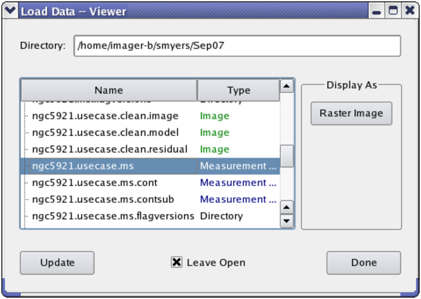
Visibility data can also be displayed and flagged directly from the task msview. Task msview allows the user to select data before it is loaded into the GUI and displayed. A screenshot is shown in Data Selection in msview. Selection parameters are field, spectral window, time range, uv range, antenna, corr, scan, array, and ms selection expression in the usual CASA selection syntax (see Data Selection).]
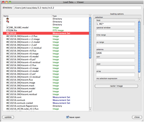
For MeasurementSet files the only option for display is ‘Raster’ (similar to AIPS task TVFLG). An example of MS display is shown in Data Display Options; loading of an MS is shown in Loading a MeasurementSet.
Warning: Only one MS should be registered at a time on a Display Panel. Only one MS can be shown in any case. You do not have to close other images/MSs, but you should at least ‘unregister’ them from the Display Panel used for viewing the MS. If you wish to see other images or MSs at the same time, create multiple Display Panel windows.
Data Display Options Panel for MeasurementSets
The Data Display Options panel provides adjustments for MSs similar to those for images, and also includes flagging options. As with images, this window appears when you choose the Data:Adjust menu or use the wrench icon from the Main Toolbar. It is also shown by default when an MS is loaded. The right panel of Data Display Options shows a Data Options window. It has a tab for each open MS, containing a set of categories. The options within each category can be either ‘rolled up’ or expanded by clicking the category label.
For a MeasurementSet, the categories are:
Advanced
MS and Visibility Selection
Display Axes
Flagging Options
Basic Settings
Axis Drawing and Labels
Color Wedge
MS Options — Basic Settings
The Basic Settings roll-up is expanded by default. It contains entries similar to those for a raster image, Data Display Options - Basic Settings). Together with the brightness/contrast and colormap adjustment icons on the Mouse Toolbar of the Display Panel, they are especially important for adjusting the color display of your MS.
The available Basic options are:
Data minimum/maximum
This has the same usage as for raster images. Lowering the data maximum will help brighten weaker data values.
Scaling power cycles
This has exactly the same usage as for raster images (see Data Display Options - Basic Settings). Again, lowering this value often helps make weaker data visible. If you want to view several fields with very different amplitudes simultaneously, this is typically one of the best adjustments to make early, together with the Colormap fiddling mouse tool, which is on the middle mouse button by default.
Colormap
Greyscale or Hot Metal colormaps are generally good choices for MS data.
MS Options— MS and Visibility Selections
Visibility Type
Visibility Component
Moving Average Size
This roll-up provides choice boxes for Visibility Type (Observed, Corrected, Model, Residual) and Component (Amplitude, Phase, Real, or Imaginary).
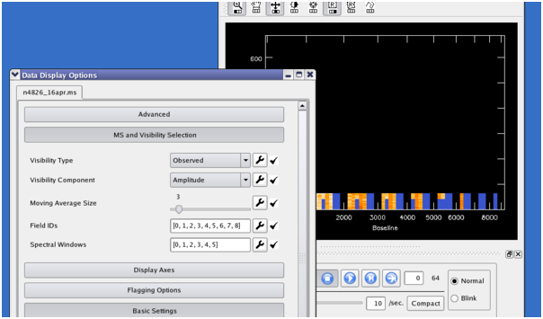
Changes to Visibility Type or Component (changing from Phase to Amplitude, for example) require the data to be retrieved again from the disk into memory, which can be a lengthy process. When a large MS is first selected for viewing, the user must trigger this retrieval manually by pressing the Apply button (located below all the options), after selecting the data to be viewed (see Field IDs and Spectral Windows, below).
Tip: Changing visibility type between ‘Observed’ and ‘Corrected’ can also be used to assure that data and flags are reloaded from disk. You should do this if you’re using another flagging tool such as autoflag simultaneously, so that msview sees the other tool’s new edits and doesn’t overwrite them with obsolete flags. The Apply button alone won’t reload unless something within msview itself requires it; in the future, a button will be provided to reload flags from the disk unconditionally.
You can also choose to view the difference from a running mean or the local RMS deviation of either Phase or Amplitude. There is a slider for choosing the nominal number of time slots in the ‘local neighborhood’ for these displays.
(Note: Insufficient Data is shown in the tracking area during these displays when there is no other unflagged data in the local neighborhood to compare to the point in question. The moving time windows will not extend across changes in either field ID or scan number boundaries, so you may see this message if your scan numbers change with every time stamp. An option will be added later to ignore scan boundaries).
Field IDs
Spectral Windows
You can retrieve and edit a selected portion of the MS data by entering the desired Spectral Window and Field ID numbers into these boxes.
Important: Especially with large MSs, often the first thing you’ll want to do is to select spectral windows which all have the same number of channels and the same polarization setup. It also makes sense to edit only a few fields at a time. Doing this will also greatly reduce data retrieval times and memory requirements.
You can separate the ID numbers with spaces or commas; you do not need to enter enclosing brackets. Changes to either entry box will cause the selected MS data to be reloaded from disk.
If you select, say, spectral windows 7, 8, 23, and 24, the animator, slice position sliders, and axis labeling will show these as 0, 1, 2, and 3 (the ‘slice positions’ or ‘pixel coordinates’ of the chosen spectral windows). Looking at the position tracking display is the best way to avoid confusion in such cases. It will show something like: Sp Win 23 (s 2) when you are viewing spectral window 23 (plane 2 of the selected spectral windows).
Changes to MS selections will not be allowed until you have saved (or discarded) any previous edits you have made (see Flagging Options – Save Edits, below). A warning is printed on the console (not the logger).
Initially, all fields and spectral windows are selected. To revert to this ‘unselected’ state, choose ‘Original’ under the wrench icons next to the entry boxes.
See MeasurementSet Visibility Selections for an example showing the use of the MS and Visibility Selections controls when viewing an MS.
MS Options — Display Axes
This roll-up is very similar to that for images: it allows the user to choose which axes (from Time, Baseline, Polarization, Channel, and Spectral Window) are on the display and the animator. There are also sliders here for choosing positions on the remaining axes. (It’s useful to note that the data is actually stored internally in memory as an array with these five axes).
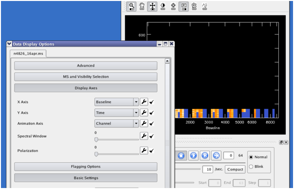
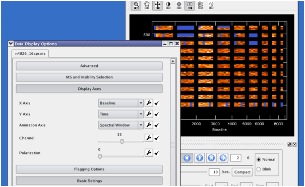
Within the Display Axes rollup you may also select whether to order the baseline axis by antenna1-antenna2 (the default) or by (unprojected) baseline length.
See MeasurementSet Display Axes–Changing the Axis of a MeasurementSet showing the use of the Display Axes controls to change the axes on the animation and sliders.
MS Options — Flagging Options
These options allow you to edit (flag or unflag) MS data. The Point Tool and Rectangle Region Mouse Tools are used on the display to select the area to edit. When using the Rectangle Region tool, double-click inside the selected rectangle to confirm the edit.
The options below determine how edits will be applied.
Show Flagged Regions…
You have the option to display flagged regions in the background color (as in TVFLG) or to highlight them with color. In the former case, flagged regions look just like regions of no data. With the (default) color option, flags are shown in shades of blue: darker blue for flags already saved to disk, lighter blue for new flags not yet saved; regions with no data will be shown in black.
Flag or Unflag
This setting determines whether selected regions will be flagged or unflagged. This does not affect previous edits; it only determines the effect which later edits will have. Both flagging and unflagging edits can be accumulated and then saved in one pass through the MS.
Flag/Unflag All…
These flagging extent checkboxes allow you to extend your edit over any of the five data axes. For example, to flag all the data in a given time range, you would check all the axes except Time, and then select the desired time range with the Rectangle Region mouse tool. Such edits will extend along the corresponding axes over the entire selected MS (whether loaded into memory or not) and optionally over unselected portions of the MS as well (Use Entire MS, below). Use care in selecting edit extents to assure that you’re editing all the data you wish to edit.
Flag/Unflag Entire Antenna?
This control can be used to extend subsequent edits to all baselines which include the desired antenna[s]. For example, if you set this item to ‘Yes’ and then click the point tool on a visibility position with baseline 3-19, the edit would extend over baselines 0-3, 1-3, 2-3, 3-3, 3-4, … 3-]nAntennas-1. Note that the second antenna of the selection (19) is irrelevant here – you can click anywhere within the ‘Antenna 3 block’, i.e., where the first antenna number is 3, to select all baselines which include antenna 3.
This item controls the edit extent only along the baseline axis. If you wish to flag all the data for a given antenna, you must still check the boxes to flag all Times, Channels, Polarizations and Spectral Windows. There would be no point, however, in activating both this item and the ‘Flag All Baselines’ checkbox. You can flag an antenna in a limited range of times, etc., by using the appropriate checkboxes and selecting a rectangular region of visibilities with the mouse.
Note: You do not need to include the entire ‘antenna block’ in your rectangle (and you may stray into the next antenna if you try). Anywhere within the block will work. To flag higher-numbered antennas, it often helps to zoom in.
Undo Last Edit
Undo All Edits
The ‘Undo’ buttons do the expected thing: completely undo the effect of the last edit (or all unsaved edits). Please note, however, that only unsaved edits can be undone here; there is no ability to revert to the flagging state at the start of the session once flags have been saved to disk (unless you have previously saved a ‘flag version’. The flag version tool is not available through msview directly).
Use Entire MS When Saving Edits?
“Yes” means that saving the edits will flag/unflag over the entire MS, including fields (and possibly spectral windows) which are not currently selected for viewing. Specifically, data within time range(s) you swept out with the mouse (even for unselected fields) will be edited.
In addition, if “Flag/Unflag All…” boxes were checked, such edits will extend throughout the MS. Note that only unselected times (fields) can be edited without checking extent boxes for the edits as well. Unselected spectral windows, e.g., will not be edited unless the edit also has “Flag/Unflag All Spectral Windows” checked.
Warning: Beware of checking “All Spectral Windows” unless you have also checked “All Channels” or turned “Entire MS” off; channel edits appropriate to the selected spectral windows may not be appropriate to unselected ones. Set “Use Entire MS” to “No” if your edits need to apply only to the portion of the MS you have selected for viewing. Edits can often be saved significantly faster this way as well. Also note that checkboxes apply to individual edits, and must be checked before making the edit with the mouse. “Use Entire MS”, on the other hand, applies to all the edits saved at one time, and must be set as desired before pressing “Save Edits”.
Save Edits
MS editing works like a text editor in that you see all of your edits immediately, but nothing is committed to disk until you press “Save Edits”. Feel free to experiment with all the other controls; nothing but ‘Save Edits’ will alter your MS on disk. As mentioned previously, however, there is no way to undo your edits once they are saved, except by manually entering the reverse edits (or restoring a previously-saved ‘flag version’).
Also, you must save (or discard) your edits before changing the MS selections. If edits are pending, the selection change will not be allowed, and a warning will appear on the console.
If you close the MS in msview, unsaved edits are simply discarded, without prior warning. It’s important, therefore, to remember to save them yourself. You can distinguish unsaved flags (when using the ‘Flags In Color’ option), because they are in a lighter shade of blue.
The program must make a pass through the MS on disk to save the edits. This can take a little time; progress is shown in the console window.
MS Options— Advanced
These settings can help optimize your memory usage, especially for large MSs. A rule of thumb is that they can be increased until response becomes sluggish, when they should be backed down again.
You can run the unix ‘top’ program and hit ‘M’ in it (to sort by memory usage) in order to examine the effects of these settings. Look at the amount of RSS (main memory) and SWAP used by the X server and ‘casaviewer’ processes. If that sounds familiar and easy, then fiddling with these settings is for you. Otherwise, the default settings should provide reasonable performance in most cases.
Cache size
The value of this option specifies the maximum number of different views of the data to save so that they can be redrawn quickly. If you run an animation or scroll around zoomed data, you will notice that the data displays noticeably faster the second time through because of this feature. Often, setting this value to the number of animation frames is ideal Note, however, that on multi-panel displays, each panel counts as one cached image.
Large images naturally take more room than small ones. The memory used for these images will show up in the X server process. If you need more Visibility Memory (below) for a really large ms, it is usually better to forgo caching a large number of views.
Max. Visibility Memory
This option specifies how many megabytes of memory may be used to store visibility data from the MeasurementSet internally. Even if you do not adjust this entry, it is useful to look at it to see how many megabytes are required to store your entire (selected) MS in memory. If the slider setting is above this, the whole selected MS will fit into the memory buffer. Otherwise, some data planes will be ‘grayed out’ (see MS Options - Apply Button), and the selected data will have to be viewed one buffer at a time, which is somewhat less convenient. In most cases, this means you should select fewer fields or spectral windows – see MS Options - MS and Visibility Selections. The ‘casaviewer’ process contains this buffer memory, which can take most of the space.
MS Options — Apply Button
When viewing large MSs the display may be partially or completely grey in areas where the required data is not currently in memory, either because no data has been loaded yet, or because not all the selected data will fit into the allowed memory (see Max. Visibility Memory above). When the cursor is over such an area, the following message shows in the position tracking area:
press 'Apply' on Adjust panel to load data
Pressing the Apply button (which lies below all the options) will reload the memory buffer so that it includes the slice you are trying to view.
The message No Data has a different meaning; in that case, there simply is no data in the selected MS at the indicated position.
For large MeasurementSets, loading visibility data into memory is the most time-consuming step. Progress feedback is provided in the console window. Again, careful selection of the data to be viewed can greatly speed up retrieval.