tclean¶

tclean(vis, selectdata=True, field='', spw='', timerange='', uvrange='', antenna='', scan='', observation='', intent='', datacolumn='corrected', imagename='', imsize=[100], cell=['1arcsec'], phasecenter='', stokes='I', projection='SIN', startmodel='', specmode='mfs', reffreq='', nchan=- 1, start='', width='', outframe='LSRK', veltype='radio', restfreq='', interpolation='linear', perchanweightdensity=True, gridder='standard', facets=1, psfphasecenter='', wprojplanes=1, vptable='', mosweight=True, aterm=True, psterm=False, wbawp=True, conjbeams=False, cfcache='', usepointing=False, computepastep=360.0, rotatepastep=360.0, pointingoffsetsigdev='', pblimit=0.2, normtype='flatnoise', deconvolver='hogbom', scales='', nterms=2, smallscalebias=0.0, restoration=True, restoringbeam='', pbcor=False, outlierfile='', weighting='natural', robust=0.5, noise='1.0Jy', npixels=0, uvtaper=[''], niter=0, gain=0.1, threshold=0.0, nsigma=0.0, cycleniter=- 1, cyclefactor=1.0, minpsffraction=0.05, maxpsffraction=0.8, interactive=False, usemask='user', mask='', pbmask=0.0, sidelobethreshold=3.0, noisethreshold=5.0, lownoisethreshold=1.5, negativethreshold=0.0, smoothfactor=1.0, minbeamfrac=0.3, cutthreshold=0.01, growiterations=75, dogrowprune=True, minpercentchange=- 1.0, verbose=False, fastnoise=True, restart=True, savemodel='none', calcres=True, calcpsf=True, psfcutoff=0.35, parallel=False)[source]¶

Radio Interferometric Image Reconstruction

[Description] [Examples] [Development] [Details]

Parameters

vis (string) - Name of input visibility file(s)
selectdata (bool=True) - Enable data selection parameters
selectdata = True
- field (string=’’) - field(s) to select
- spw (string=’’) - spw(s)/channels to select
- timerange (string=’’) - Range of time to select from data
- uvrange (string=’’) - Select data within uvrange
- antenna (string=’’) - Select data based on antenna/baseline
- scan (string=’’) - Scan number range
- observation (string=’’) - Observation ID range
- intent (string=’’) - Scan Intent(s)
datacolumn (string=’corrected’) - Data column to image(data,corrected)
imagename (string=’’) - Pre-name of output images
imsize (intVec=[100]) - Number of pixels
cell (stringVec=[“1arcsec”]) - Cell size
phasecenter (string=’’) - Phase center of the image
stokes (string=’I’) - Stokes Planes to make
projection (string=’SIN’) - Coordinate projection
startmodel (string=’’) - Name of starting model image
specmode (string=’mfs’) - Spectral definition mode (mfs,cube,cubedata, cubesource)
specmode = mfs
- reffreq (string=’’) - Reference frequency
specmode = cube
- nchan (int=-1) - Number of channels in the output image
- start (string=’’) - First channel (e.g. start=3,start='1.1GHz',start='15343km/s')
- width (string=’’) - Channel width (e.g. width=2,width='0.1MHz',width='10km/s')
- outframe (string=’LSRK’) - Spectral reference frame in which to interpret 'start' and 'width'
- veltype (string=’radio’) - Velocity type (radio, z, ratio, beta, gamma, optical)
- restfreq (stringVec=’’) - List of rest frequencies
- interpolation (string=’linear’) - Spectral interpolation (nearest,linear,cubic)
- perchanweightdensity (bool=True) - whether to calculate weight density per channel in Briggs style weighting or not
specmode = cubesource
- nchan (int=-1) - Number of channels in the output image
- start (string=’’) - First channel (e.g. start=3,start='1.1GHz',start='15343km/s')
- width (string=’’) - Channel width (e.g. width=2,width='0.1MHz',width='10km/s')
- outframe (string=’LSRK’) - Spectral reference frame in which to interpret 'start' and 'width'
- veltype (string=’radio’) - Velocity type (radio, z, ratio, beta, gamma, optical)
- restfreq (stringVec=’’) - List of rest frequencies
- interpolation (string=’linear’) - Spectral interpolation (nearest,linear,cubic)
- perchanweightdensity (bool=True) - whether to calculate weight density per channel in Briggs style weighting or not
specmode = cubedata
- nchan (int=-1) - Number of channels in the output image
- start (string=’’) - First channel (e.g. start=3,start='1.1GHz',start='15343km/s')
- width (string=’’) - Channel width (e.g. width=2,width='0.1MHz',width='10km/s')
- veltype (string=’radio’) - Velocity type (radio, z, ratio, beta, gamma, optical)
- restfreq (stringVec=’’) - List of rest frequencies
- interpolation (string=’linear’) - Spectral interpolation (nearest,linear,cubic)
- perchanweightdensity (bool=True) - whether to calculate weight density per channel in Briggs style weighting or not
gridder (string=’standard’) - Gridding options (standard, wproject, widefield, mosaic, awproject)
gridder = standard
- vptable (string=’’) - Name of Voltage Pattern table
- pblimit (double=0.2) - PB gain level at which to cut off normalizations
gridder = widefield
- wprojplanes (int=1) - Number of distinct w-values for convolution functions
- facets (int=1) - Number of facets on a side
- vptable (string=’’) - Name of Voltage Pattern table
- pblimit (double=0.2) - PB gain level at which to cut off normalizations
gridder = wproject
- wprojplanes (int=1) - Number of distinct w-values for convolution functions
- vptable (string=’’) - Name of Voltage Pattern table
- pblimit (double=0.2) - PB gain level at which to cut off normalizations
gridder = wprojectft
- wprojplanes (int=1) - Number of distinct w-values for convolution functions
- vptable (string=’’) - Name of Voltage Pattern table
- pblimit (double=0.2) - PB gain level at which to cut off normalizations
gridder = mosaic
- normtype (string=’flatnoise’) - Normalization type (flatnoise, flatsky,pbsquare)
- vptable (string=’’) - Name of Voltage Pattern table
- usepointing (bool=False) - The parameter makes the gridder utilize the pointing table phase directions while computing the residual image.
- mosweight (bool=True) - Indepently weight each field in a mosaic
- pblimit (double=0.2) - PB gain level at which to cut off normalizations
- conjbeams (bool=False) - Use conjugate frequency for wideband A-terms
- psfphasecenter (string=’’) - optional direction to calculate psf for mosaic (default is image phasecenter)
gridder = mosaicft
- normtype (string=’flatnoise’) - Normalization type (flatnoise, flatsky,pbsquare)
- vptable (string=’’) - Name of Voltage Pattern table
- usepointing (bool=False) - The parameter makes the gridder utilize the pointing table phase directions while computing the residual image.
- pblimit (double=0.2) - PB gain level at which to cut off normalizations
- conjbeams (bool=False) - Use conjugate frequency for wideband A-terms
- psfphasecenter (string=’’) - optional direction to calculate psf for mosaic (default is image phasecenter)
gridder = ftmosaic
- normtype (string=’flatnoise’) - Normalization type (flatnoise, flatsky,pbsquare)
- vptable (string=’’) - Name of Voltage Pattern table
- usepointing (bool=False) - The parameter makes the gridder utilize the pointing table phase directions while computing the residual image.
- mosweight (bool=True) - Indepently weight each field in a mosaic
- pblimit (double=0.2) - PB gain level at which to cut off normalizations
gridder = imagemosaic
- wprojplanes (int=1) - Number of distinct w-values for convolution functions
- normtype (string=’flatnoise’) - Normalization type (flatnoise, flatsky,pbsquare)
- vptable (string=’’) - Name of Voltage Pattern table
- pblimit (double=0.2) - PB gain level at which to cut off normalizations
gridder = awproject
- wprojplanes (int=1) - Number of distinct w-values for convolution functions
- normtype (string=’flatnoise’) - Normalization type (flatnoise, flatsky,pbsquare)
- psterm (bool=False) - Use prolate spheroidal during gridding
- aterm (bool=True) - Use aperture illumination functions during gridding
- cfcache (string=’’) - Convolution function cache directory name
- computepastep (double=360.0) - Parallactic angle interval after the AIFs are recomputed (deg)
- rotatepastep (double=360.0) - Parallactic angle interval after which the nearest AIF is rotated (deg)
- pointingoffsetsigdev (doubleVec=’’) - Pointing offset threshold to determine heterogeneity of pointing corrections for the AWProject gridder
- wbawp (bool=True) - Use wideband A-terms
- mosweight (bool=True) - Indepently weight each field in a mosaic
- pblimit (double=0.2) - PB gain level at which to cut off normalizations
- conjbeams (bool=False) - Use conjugate frequency for wideband A-terms
- usepointing (bool=False) - The parameter makes the gridder utilize the pointing table phase directions while computing the residual image.
gridder = awprojectft
- wprojplanes (int=1) - Number of distinct w-values for convolution functions
- normtype (string=’flatnoise’) - Normalization type (flatnoise, flatsky,pbsquare)
- psterm (bool=False) - Use prolate spheroidal during gridding
- aterm (bool=True) - Use aperture illumination functions during gridding
- cfcache (string=’’) - Convolution function cache directory name
- computepastep (double=360.0) - Parallactic angle interval after the AIFs are recomputed (deg)
- rotatepastep (double=360.0) - Parallactic angle interval after which the nearest AIF is rotated (deg)
- pointingoffsetsigdev (doubleVec=’’) - Pointing offset threshold to determine heterogeneity of pointing corrections for the AWProject gridder
- wbawp (bool=True) - Use wideband A-terms
- mosweight (bool=True) - Indepently weight each field in a mosaic
- pblimit (double=0.2) - PB gain level at which to cut off normalizations
- conjbeams (bool=False) - Use conjugate frequency for wideband A-terms
- usepointing (bool=False) - The parameter makes the gridder utilize the pointing table phase directions while computing the residual image.
deconvolver (string=’hogbom’) - Minor cycle algorithm (hogbom,clark,multiscale,mtmfs,mem,clarkstokes)
deconvolver = multiscale
- scales (intVec=’’) - List of scale sizes (in pixels) for multi-scale algorithms
- smallscalebias (double=0.0) - Biases the scale selection when using multi-scale or mtmfs deconvolvers
deconvolver = mtmfs
- scales (intVec=’’) - List of scale sizes (in pixels) for multi-scale algorithms
- nterms (int=2) - Number of Taylor coefficients in the spectral model
- smallscalebias (double=0.0) - Biases the scale selection when using multi-scale or mtmfs deconvolvers
restoration (bool=True) - Do restoration steps (or not)
restoration = True
- restoringbeam (stringVec=’’) - Restoring beam shape to use. Default is the PSF main lobe
- pbcor (bool=False) - Apply PB correction on the output restored image
outlierfile (string=’’) - Name of outlier-field image definitions
weighting (string=’natural’) - Weighting scheme (natural,uniform,briggs, briggsabs[experimental], briggsbwtaper[experimental])
weighting = natural
- uvtaper (stringVec=[‘’]) - uv-taper on outer baselines in uv-plane
weighting = briggs
- robust (double=0.5) - Robustness parameter
- npixels (int=0) - Number of pixels to determine uv-cell size
- uvtaper (stringVec=[‘’]) - uv-taper on outer baselines in uv-plane
weighting = briggsabs
- robust (double=0.5) - Robustness parameter
- noise (variant=’1.0Jy’) - noise parameter for briggs abs mode weighting
- npixels (int=0) - Number of pixels to determine uv-cell size
- uvtaper (stringVec=[‘’]) - uv-taper on outer baselines in uv-plane
weighting = briggsbwtaper
- robust (double=0.5) - Robustness parameter
- uvtaper (stringVec=[‘’]) - uv-taper on outer baselines in uv-plane
niter (int=0) - Maximum number of iterations
niter != 0
- gain (double=0.1) - Loop gain
- threshold (double=0.0) - Stopping threshold
- nsigma (double=0.0) - Multiplicative factor for rms-based threshold stopping
- cycleniter (int=-1) - Maximum number of minor-cycle iterations
- cyclefactor (double=1.0) - Scaling on PSF sidelobe level to compute the minor-cycle stopping threshold.
- minpsffraction (double=0.05) - PSF fraction that marks the max depth of cleaning in the minor cycle
- maxpsffraction (double=0.8) - PSF fraction that marks the minimum depth of cleaning in the minor cycle
- interactive (bool=False) - Modify masks and parameters at runtime
usemask (string=’user’) - Type of mask(s) for deconvolution: user, pb, or auto-multithresh
usemask = user
- mask (string=’’) - Mask (a list of image name(s) or region file(s) or region string(s) )
- pbmask (double=0.0) - primary beam mask
usemask = pb
- pbmask (double=0.0) - primary beam mask
usemask = auto-multithresh
- pbmask (double=0.0) - primary beam mask
- sidelobethreshold (double=3.0) - sidelobethreshold * the max sidelobe level * peak residual
- noisethreshold (double=5.0) - noisethreshold * rms in residual image + location(median)
- lownoisethreshold (double=1.5) - lownoisethreshold * rms in residual image + location(median)
- negativethreshold (double=0.0) - negativethreshold * rms in residual image + location(median)
- smoothfactor (double=1.0) - smoothing factor in a unit of the beam
- minbeamfrac (double=0.3) - minimum beam fraction for pruning
- cutthreshold (double=0.01) - threshold to cut the smoothed mask to create a final mask
- growiterations (int=75) - number of binary dilation iterations for growing the mask
- dogrowprune (bool=True) - Do pruning on the grow mask
- minpercentchange (double=-1.0) - minimum percentage change in mask size (per channel plane) to trigger updating of mask by automask
- verbose (bool=False) - True: print more automasking information in the logger
fastnoise (bool=True) - True: use the faster (old) noise calculation. False: use the new improved noise calculations
restart (bool=True) - True : Re-use existing images. False : Increment imagename
savemodel (string=’none’) - Options to save model visibilities (none, virtual, modelcolumn)
calcres (bool=True) - Calculate initial residual image
calcpsf (bool=True) - Calculate PSF
calcpsf = True
- psfcutoff (double=0.35) - All pixels in the main lobe of the PSF above psfcutoff are used to fit a Gaussian beam (the Clean beam).
parallel (bool=False) - Run major cycles in parallel

Description

tclean handles continuum images and spectral line cubes, full Stokes polarization imaging, supports outlier fields, contains point-source CLEAN based algorithms as well as options for multi-scale and wideband image reconstruction , widefield imaging correcting for the w-term, full primary-beam imaging and joint mosaic imaging (with heterogeneous array support for ALMA). Parallelization of the major cycle is also available.

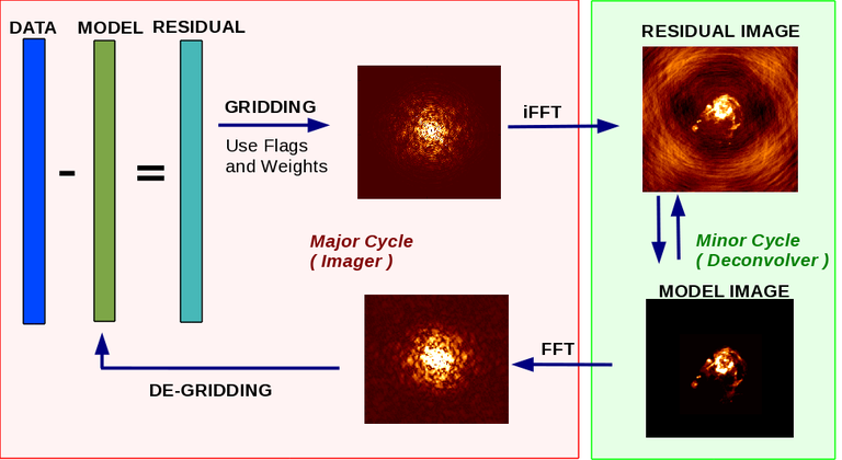
The tclean task as based on the CLEAN algorithm , which is the most popular and widely-studied method for reconstructing a model image based on interferometer data. It iteratively removes at each step a fraction of the flux in the brightest pixel in a defined region of the current “dirty” image, and places this in the model image.

Image reconstruction in CASA typically comprises an outer loop of major cycles and an inner loop of minor cycles. The major cycle implements transforms between the data and image domains and the minor cycle operates purely in the image domain. Together, they implement an iterative weighted \(\chi^2\) minimization that solves the measurement equation. Minor cycle algorithms can have their own (different) optimization schemes and the imaging framework and task interface allow for considerable freedom in choosing options separately for each step of the process.

../../_images/26ad14d4f63ff633dbd5d9e92d40a5059ab46a67.png

Operating Modes

The tclean task can be configured to perform either full iterative image reconstructions (see synthesis-imaging ) or to run each step separately. Parameters for data selection, image definition, gridding and deconvolution algorithms, restoration and primary beam setup are shared between all operational modes.

The main usage modes of tclean are:

Imaging and Deconvolution Iterations:

Construct the PSF and Dirty image and apply a deconvolution algorithm to reconstruct a Sky model. A series of major and minor cycle iterations are usually performed. The output sky model is then restored and optionally PB-corrected. The Sky model can optionally be saved in the MS during the last major cycle.

Make PSF and PB:

Make only the Point Spread Function and the Primary Beam, along with auxiliary weight images (a single pixel image containing sum-of-weight per plane, and (for mosaic and aprojection) a weight image containing the weighted sum of PB square).

Make a Residual/Dirty Image:

Make a dirty image, or a new residual image using an existing or specified model image. This step requires the presence of the sum-of-weight and weight images (for normalization) constructed during the PSF and PB generation step.

Model Prediction:

Save a sky model in the MeasurementSet for later use in calibration (virtual model or by actual prediction into a model column).

When savemodel=’modelcolumn’ is chosen, the message, “Saving model column” will appear in the logger during the last major cycle. The model will be written to MODEL_DATA column of the main table of the MS for relevant field and spw(s). Similarly, with savemodel=‘virtual’, the message, “Saving virtual model” will appear in the logger. In the case of the virtual model, the model parameters are saved in a keyword of the main table in the MS or in SOURCE subtable. SOURCE subtable is an optional table and if it exists and containing non-zero number of rows, the model parameters are written to SOURCE_MODEL column in the row for the corresponding SOURCE ID. When the virtual model is stored in the keyword of the MS, they are stored with key name such as ‘model_0’. In the case of multiple models exist, say for multiple fields, one can associate particular model key name with a specific field id by looking up the key, ‘definedmodel_field_#’, where # is the field id. Additional information is avaialbe at Virtual Model Visibilities.

To check if model visibility data is present in the MS,

tb.open('xxx.ms')
tb.colnames()  # will show MODEL_DATA in the the returned column names if MODEL_DATA column exists
tb.keywordnames() # if you see, definedmodel_field_{fieldid}, there is a virtual model exists for the field 
# Also the model parameters (e.g. for 'model_0') can be retrieved by
mymodel=tb.getkeyword('model_0')
tb.done()

# If SOURCE is listed in the keywordnames listing in the above command, and if SOURCE has non-zero rows, virtual model(s) 
# may exist in SOURCE_MODEL column of SOURCE, 
# e.g. to get a virutal model for field id=0 (source id=0)
tb.open('xxx.ms/SOURCE')
mymodel=tb.getcell('SOURCE_MODEL',0)   # note that since the model parameter are stored in the record (Python dictionaruy)tb.getcol cannot be used)
tb.done()

To check the content of the model data ( either from MODEL_DATA or virutal model generated on the fly),

plotms(vis=‘xxx.ms’, field=‘your_field_that_model_expected_to_be_stored’, spw=.., xaxis=‘uvidist’, yaxis=‘amp’,ydatacolumn=‘model’)

Warning

Please note that tclean may be safely interrupted using a Ctrl-C at all times except when it is in the middle of writing the model data column during a major cycle. To avoid concerns about corrupting your MS by trying to interrupt tclean during a disk write, please run image-reconstruction and model-saving in two separate steps, with model writing turned off during the iterative image reconstruction step. For example:

tclean(vis='xxx.ms', imagename='try',......., niter=20,savemodel='none')
tclean(vis='xxx.ms', imagename='try',...., niter=0, savemodel='modelcolumn', calcpsf=False, calcres=False, restoration=False)

This sequence will show a message in the logger that says “Saving Model Column”. Note that while this “predict-only” major cycle is ongoing, Ctrl-C should not be used.

PB-Correction:

Divide out the Primary Beam from the restored Sky image.

pblimit

The pblimit is a parameter used to define the value of the antenna primary beam gain, below which wide-field gridding algorithms such as ‘mosaic’ and ‘awproject’ will not apply normalization (and will therefore set to zero). For gridder=’standard’, ‘wproject’ , ‘widefield’ there is no pb-based normalization during gridding and so the absolute value of this parameter is ignored.

The sign of the pblimit parameter is used for a different purpose. If positive, it defines a T/F pixel mask that is attached to the output residual and restored images. If negative, this T/F pixel mask is not included. For the ‘mosaic’ and ‘awproject’ gridders, the zeros in the regions outside the absolute pblimit level will be visible without the T/F mask, and for other gridders that do not do any pblimit-based normalizations (‘standard’, ‘wproject’, ‘widefield’) those regions will contain valid image pixels.

Please note that this pixel mask is different from the deconvolution mask used to control the region where CLEAN based algorithms will search for source peaks. In order to set a deconvolution mask based on pb level, please use the ‘pbmask’ parameter.

Warning

Certain values of pblimit should be avoided! These values are 1, -1, and 0. Details can be found here.

widebandpbcor

Widebandpbcor is a separate task, and will eventually be implemented as a parameter in tclean. It allows correction of the primary beam as part of wideband imaging. It computes a set of PBs at the specified frequencies, calculates Taylor-coefficient images that represent the PB spectrum, performs a polynomial division to PB-correct the output Taylor-coefficient images from tclean (with nterms>1 and deconvolver=’mtmfs’), and recomputes the spectral index (and curvature) using the PB-corrected Taylor-coefficient images.

Pointing Corrections:

Heterogeneous Pointing Corrections can optionally be applied with the usepointing and pointingoffsetsigdev parameters. These parameters apply corrections based on the pointing errors that are present in the POINTING sub-table. This can improve imaging performance for observations with high wide-band sensitivity, such as is typically observed with the VLA and ALMA telescopes. An overview of pointing corrections is given in the CASA Docs page on Widefield Imaging.

Restoration:

Specify a restoring beam and re-restore the model image.

Auto-masking:

Automatically mask emission during clean; see Masks for Deconvolution for more information.

Output Images

Depending on the operation being run, a subset of the following output images will be written to disk.

imagename = ‘try’

try.psf	Point Spread Function
try.pb	Primary Beam
try.residual	Residual Image (or initial Dirty Image)
try.model	Model Image after deconvolution
try.image	Restored output image
try.image.pbcor	Primary Beam corrected image
try.mask	Deconvolution mask
try.sumwt	A single pixel image containing sum of weights per plane
try.weight	Image of un-normalized sum of PB-square (for mosaics and A-Projection)
try.psf.tt0, try.psf.tt1, try.psf.tt2, try.model.tt0, try.model.tt1, try.residual.tt0, try.residual.tt1, try.image.tt0, try.image.tt1, etc…	Multi-term images representing Taylor coefficients (of polynomials that model the sky spectrum)
try.alpha	Spectral index, for multi-term wideband imagging
try.alpha.error	Estimate of error on spectral index
try.beta	Spectral curvature for multi-term wideband images (if nterms > 2)
try_1., try_2., try_3.*, etc.	Auto-incremented image names when restart=False
try1_1., try1_2., try1_3.*, etc.	Auto-incremented image names with multiple fields when restart=False
try.workdirectory ( try.n1.psf, try.n2.psf, try.n3.psf, try.n1.residual, try.n2.residual, try.n3.residual, try.n1.weight, try.n2.weight, try.n3.weight, try.n1.gridwt, try.n2.gridwt, etc… )	Scratch images written within a ‘work directory’ for parallel imaging runs for cube imaging. The reference images are reference-concatenated at the end to produce single output cubes. As of CASA 5.7, continuum imaging no longer produces a try.workdirectory.

Warning

If an image with that name already exists, it will in general be overwritten. Beware using names of existing images however. If the tclean is run using an imagename where <imagename>.residual and <imagename>.model already exist, then tclean will continue starting from these (effectively restarting from the end of the previous tclean). Thus, if multiple runs of tclean are run consecutively with the same imagename, then the cleaning is incremental.

Tip

To organize the output images produced by one or multiple runs of tclean and/or other imaging tasks, a subdirectory can be added to ‘imagename’. All output images will be sent to that directory instead of the current working directory. Example: imagename=’mydir/try’. This is a simple way to group together a set of images (different extensions) corresponding to a same sequence of tclean runs, preventing confusion and conflicts with the potentially long list of other images from related or unrelated tclean runs that used similar ‘imagename’.

Stokes polarization products

It is possible to make polarization images of various Stokes parameters, based on the R/L circular (e.g., VLA) or the X/Y linear (e.g., ALMA) polarization products. When specifying multiple values in the ‘stokes’ parameter, the output image will have planes (along the “polarization” axis) corresponding to the chosen Stokes parameters.

The Stokes parameter is specified as a string of up to four letters, and can indicate stokes parameters themselves, Right/Left hand polarization products, or linear polarization products (X/Y). Examples include:

stokes = 'I' # Intensity only (default)
stokes = 'IQU' # Intensity and linear polarization
stokes = 'IV' # Intensity and circular polarization
stokes = 'IQUV' # All Stokes imaging
stokes = 'RR' # Right hand polarization only
stokes = 'XXYY' # Both linear polarizations
stokes = 'pseudoI' # Intensity only, but including data with one of the parallel polarizations flagged

For imaging the total intensity, the stokes=’I’ option is stricter than the stokes=’pseudoI’ option in the sense that it excludes all correlations for which any correlation is flagged, even though the remaining correlations are valid. On the other hand, the’pseudoI’option allows Stokes I images to include data for which either of the parallel hand data are unflagged. For example, if you have RR and LL dual polarization data and you flagged parts of RR but not LL, stokes=’I’ will ignore both polarizations in the time-stamps where RR are flagged, while stokes=’pseudoI’ will include all unflagged data in the total intensity image. See the CASA Docs pages on Types of Images and Single Dish Imaging (tsdimaging) for more information. It is also possible to split out a polarization product with split and image separately, but you will not be able to combine these part-flagged data in the uv-domain.

Functional Parameter Blocks

The tclean parameters are arranged in the functional blocks described below. More details on the individual parameters and sub-parameters can be found under the Parameters tab at the top of this page.

As a general rule, sub-parameters will appear (and be used) only when a parent parameter has a specific value. This means that for a given set of choices (e.g. deconvolution or gridding algorithm) only parameters that are relevant to that choice will be visible to the user when ” inp() ” is invoked. It is advised that this task interface be used even when constructing tclean scripts that call the task as a python call ” tclean(….) ” to understand which parameters are relevant to the run and which are not.

Data Selection (selectdata)

Selection parameters allow the definition of a subset of the supplied MS (or list of MSs) on which the imaging is to operate. Details can be found on the CASA Docs pages of Visibility Selection.

Image Definition (specmode)

The image coordinate system(s) and shape(s) can be set up to form single images (from a single field or from multiple fields forming a mosaic),or multiple fields. The different modes for imaging include:

‘mfs’: multi-frequency synthesis, i.e., continuum imaging with only one output image channel.
‘cube’: Spectral line imaging with one or more channels. The fixed spectral frame, LSRK, will be used for automatic internal software Doppler tracking so that a spectral line observed over an extended time range will line up appropriately.
‘cubedata’: Spectral line imaging with one or more channels There is no internal software Doppler tracking so a spectral line observed over an extended time range may be smeared out in frequency.
‘cubesource’: Spectral line imaging while tracking moving source (near field or solar system ephemeris objects ). The velocity of the source is accounted and the frequency reported is in the source frame.

Combined use of the parameters ‘specmode’ and ‘gridder’ (see below) allows to specify smaller outlier fields, facetted images, single plane wideband images (with 1 or more Taylor terms to model spectra), 3D spectral cubes with multiple channels, 3D images with multiple Stokes planes, 4D images with frequency channels and Stokes planes. Various combinations of all these options are also supported.

The CASA Docs pages on Image Types provide more details.

Gridding Options (gridder)

Options for convolutional resampling include standard gridding using a prolate spheroidal function, the use of FTs of Fresnel kernels for W-Projection, the use of baseline aperture illumination functions for A-Projection and Mosaicing. These include:

‘standard’: standard gridding using a prolate spheroidal function
‘wproject’: use of FTs of Fresnel kernels to correct for the widefield non-coplanar baseline effect (Cornwell et.al 2008)
‘widefield’: Facetted imaging with or without W-Projection per facet.
‘mosaic’: A-Projection that uses baseline, frequency and time dependent primary beams, without sidelobes, beam rotation or squint correction.
‘awproject’: A-Projection from aperture illumination models with azimuthally asymmetric beams, including beam rotation, squint correction, conjugate frequency beams and W-projection (Bhatnagar et.al, 2008).

Combinations of these options are also available. See the CASA Docs pages on Widefield Imaging for more information.

For mosaicing and AW-projection, the frequency dependence of the primary beam within the data being imaged is included in the calculations and can optionally also be corrected for during gridding. See the CASA Docs page on Wideband Imaging for details.

Deconvolution Options (deconvolver)

All our algorithms follow the Cotton-Schwab CLEAN style of major and minor cycles with the details of the deconvolution algorithm usually contained within the minor cycle and operating in the image domain. Options include:

‘hogbom’: An adapted version of Hogbom Clean (Hogbom, 1974)
‘clark’: An adapted version of Clark Clean (Clark, 1980)
‘clarkstokes’: Clark Clean operating separately per Stokes plane
‘multiscale’: MultiScale Clean (Cornwell, 2008). Scale-sensitive deconvolution algorithm designed for images with complicated spatial structure. It parameterizes the image into a collection of inverted tapered paraboloids.
‘mtmfs’: Multi-term (Multi Scale) Multi-Frequency Synthesis (Rau and Cornwell, 2011). Models the wide-band sky brightness distribution through the use of multi-term Taylor polynomial and wideband primary beam corrections (to be used with nterms>1).
‘mem’: Maximum Entropy Method (Cornwell and Evans, 1985). Note: The MEM implementation in CASA is not very robust, improvements will be made in the future.

If as input to tclean the stokes parameter includes polarization planes other than I, then choosing deconvolver=’hogbom’ or ‘clarkstokes’ will clean (search for components) each plane sequentially, while deconvolver =’clark’ will deconvolve jointly.

For more details, see the CASA Docs pages on Deconvolution Algorithms.

Several options for making masks, including automasking, are also provided.

Data Weighting (weighting)

Data weighting during imaging allows for the improvement of the dynamic range and the ability to adjust the synthesized beam associated with the produced image. The weight given to each visibility sample can be adjusted to fit the desired output. There are several reasons to adjust the weighting, including improving sensitivity to extended sources or accounting for noise variation between samples. The user can adjust the weighting by changing the weighting parameter with seven options: ‘natural’, ‘uniform’, ‘briggs’, ‘superuniform’, ‘briggsabs’, ‘briggsbwtaper’, and ‘radial’. Optionally, a UV taper can be applied, and various parameters can be set to further adjust the weight calculations.

The most used options for data weighting are ‘natural’, ‘unform’ and ‘briggs’.

‘Natural’ weighting gives equal weight to all samples, resulting in the lowest noise level and largest (poorest) resolution, with relatively high sidelobe levels.
‘Uniform’ weighting gives a weight inversely proportional to the sampling density function, which minimizes sidelobe levels and provides higher resolution, but at the expense of higher noise levels.
‘Briggs’ weighting provides a compromise between natural and uniform weighting, and often optimizes between angular resolution, noise, and sidelobe levels. The key parameter for briggs weighting is the robust sub-parameter, which takes value between -2.0 (close to uniform weighting) to 2.0 (close to natural). The scaling of Ris such that robust=0 gives a good trade-off between resolution and sensitivity.

In addition to the weighting scheme specified via the ‘weighting’ parameter, additional weights can be applied:

The ‘uvtaper’ parameter applies a Gaussian taper on the weights of the UV data, in addition to the weighting scheme specified via the ‘weighting’ parameter. It is equivalent to smoothing the PSF obtained by other weighting schemes and can be specified either as a Gaussian in uv-space (eg. units of lambda or klambda) or as a Gaussian in the image domain (eg. angular units like arcsec). The effect of uvtaper this is that the clean beam becomes larger, and surface brightness sensitivity increases for extended emission.
The ‘perchanweightdensity’ parameter (for briggs and uniform weighting of cubes) determines whether to calculate the weight density for each channel independently (True) or a common weight density for all of the selected data (False). In general, perchanweightdensity=True (default since CASA 5.5) provides more uniform sensitivity per channel for cubes, but with generally larger PSFs, while perchanweightdensity=False results in smaller psfs for the same robustness value, but the rms noise as a function of channel varies and increases toward the edge channels.
The ‘mosweight’ sub-parameter of the mosaic gridder determines whether to weight each field in a mosaic independently (mosweight = True), or to calculate the weight density from the average uv distribution of all the fields combined (mosweight = False). For ALMA it has been shown that mosweight = True (default since CASA 5.4) may give better results in the presence of poor uv-coverage or non-uniform sensitivity across the mosaic, but the downside is that the major and minor axis of the synthesized beam may be ~10% larger than with mosweight=False, and it may potentially cause memory issues for large VLA mosaics.

More details on data weighting can be found on the Image Algorithm pages of CASA Docs

Iteration Control (niter)

Iterations are controlled by user parameters (gain, niter, etc..) as well as stopping criteria that decide when to exit minor cycle iterations and trigger the next major cycle, and also when to terminate the major-minor loop. These stopping criteria include reaching iteration limits, convergence thresholds, and signs of divergence with appropriate messages displayed in the log. For more details, see the CASA Docs pages on Iteration Control .

Other Options

Handling Large Data and Image Sizes

Parallelization of the major cycle is available for continuum imaging and of both major and minor cycles for cube imaging. In order to run tclean in parallel mode it is necessary to launch CASA with mpicasa, and set the tclean parameter parallel=True. The parallelization of tclean works in the same way if the input is a normal MS or a Multi-MS (MMS), and thus differs from the parallel approach used by other tasks in that it does not require a partitioned MMS file. Details can be found in the CASA Docs chapter on Parallel Processing .

For large image cubes, the gridders can run into memory limits as they loop over all available image planes for each row of data accessed. To prevent this problem, we can grid subsets of channels in sequence with the chanchunks parameter, so that at any given time only part of the image cube needs to be loaded into memory. The chanchunks parameter controls the number of chunks to split the cube into.

User Interaction

Options for user interaction include interactive masking and editing of iteration control parameters. The output log files can also be used to diagnose some problems.

Several convenience features are also available, such as operating on the MS in read-only mode (which does not require write permissions), the ability to restart and continue imaging runs without incuring the unnecessary cost of an initial major cycle or PSF construction and the optional return of a python dictionary that contains the convergence history of the run.

Scripting Controls

Finer control can be achieved using the PySynthesisImager tools to run (for example) only image domain deconvolution or to insert methods for automatic mask generation (for example) in between the existing major/minor cycle loops or to connect external methods or algorithms for either the minor or major cycles.

Tracking moving sources or sources with ephemeris tables

If the phasecenter is a known major solar system object (‘MERCURY’, ‘VENUS’, ‘MARS’, ‘JUPITER’, ‘SATURN’, ‘URANUS’, ‘NEPTUNE’, ‘PLUTO’, ‘SUN’, ‘MOON’) or is an ephemerides table, then that source is tracked and the background sources get smeared (which is useful especially for long observations or multi epoch data). There is a special case, when phasecenter=’TRACKFIELD’, which will use the ephemerides or polynomial phasecenter in the FIELD table of the MeasurementSets as the source center to track. When in tracking mode, the image center will be the direction of the source at the first time in the user selected data. At all other times, the source will be shifted by the amount it has moved in the frame of the image to that initial time. Examples of usage are presented in the tclean examples tab.

Note

When displaying ephemeris images, it is good practice to use relative coordinates to determine the average offset of emission from the ephemeris path over the observation, i.e., axis label properties: world coordinate, relative position. The use of the absolute grid (default) can be misleading since the chosen coordinate frame is associated with the ephemeris path location at an unspecified time, although usually near the beginning of the experimient.

More information can be found in the CASA Docs chapter on Ephemeris Data.

History

At the end of a successful tclean run, the history of the output images is updated. For every tclean command a series of entries is recorded, including the task name (tclean), the CASA version used, and every parameter-value pair of the task.

The history is written to all the images associated with the current run, identified by the image base name given in the imagename parameter. This feature searches for all the images with names starting with that basename and followed by a dot-separated extension (imagename.*). In addition it also searches for imagename[INTEGERS]_[INTEGERS].*, to cover auto-incremented image names (see the table of possible image names above).

The image history entries added by tclean can be inspected using the task imhistory (see API), similarly as with the history entries added by other image analysis tasks.

As a lower level interface, the image history can be also inspected and manipulated using CASA tools such as the image analysis tool and the table tool (see API). The history entries are written into the ‘logtable’ subtable of the images.

Note

Because history is written into all the images found with the ‘imagename’ prefix and a dot-separated extension, there is a corner case where history entries can be written in images that are not related to the tclean command just executed. For example, if a first tclean command used imagename=’tst.mfs.hogbom’, and a second command uses imagename=’tst.mfs’. This can happen if the tclean commands use the same directory, the imagename string is a shorter version of a previously used imagename, and the longer name is used first and is the shorter name (to be used afterwards) followed by a dot ‘.’ and more characters. This naming scheme produces an ambiguity with the rules used to name output images (imagename + ‘.’ + multiple extensions) and is risky, as it can be very difficult for the user to anticipate all the possible conflicts and confusions with image extensions used by tclean and other imaging tasks.

Processing information

Several parameters related to runtime processing are added to the miscinfo (miscellaneous information) record of the images produced by tclean. These are technical parameters related to processes and memory use:

mpiprocs: integer, number of processes (>1 for parallel runs)
chnchnks: integer, number of sub-cubes or chanchunks into which cubes are partitioned in the major cycles
memavail: float, estimated available memory, as found by tclean at the beginning of the first major cycle.
memreq: float, estimate of memory required, as a function of cube size, number of processors, and a few heuristic scale factors. Expressed in GBs.

These parameters are added to the miscinfo record of the output images by the tclean command that creates them, and represent the runtime processing information of that command.

Similarly as with other parameters included in the miscinfo record, these are exported to FITS images by the exportfits task, if the parameter history is True. The miscinfo record can be inspected using the image tool (see API).

The same values are written to the CASA log at the beginning of every major cycle. The memreq estimate should not be interpreted as the amount of memory that tclean is going to use. It is an estimate of memory that would be required to fit all the data in memory, also accounting for the fact that that multiple processes would work on the data simultaneously if running in parallel mode.

The memreq value is used to estimate the required chnchnks or number of sub-cubes into which the data are partitioned in the major cycles. chnchnks is roughly estimated as the result from dividing memreq by memavail. The amount of memory effectively used is kept below the estimated amount of memory available, thanks to the partitioning of the data in sub-cubes and further finer partitioning done in the minor cycles. The memreq estimate grows proportionally to the data dimensions, type of gridder, and number of processes in parallel mode.

Examples

The following examples, to be expanded, highlight modes and options that the tclean task supports. The examples below are written as scripts that may be copied and pasted to get started with the basic parameters needed for a particular operation. When writing scripts, it is advised that the interactive task interface be used to view lists of sub-parameters that are relevant only to the operations being performed. For example, setting specmode=’cube’ and running inp() will list parameters that are relevant to spectral coordinate definition, or setting niter to a number greater than zero (niter=100) followed by inp() will list iteration control parameters. Note that all runs of tclean need the following parameters: vis, imagename, imsize, and cell. By default, tclean will run with niter=0, making the PSF, a primary beam, the initial dirty (or residual) image and a restored version of the image.

For examples running tclean on ALMA data, see also the CASA Guide “Tclean and ALMA”.

Imaging and Deconvolution Iterations

Using Hogbom CLEAN on a single MFS image

tclean(vis='test.ms', imagename='try1', imsize=100, cell='10.0arcsec', specmode='mfs',
       deconvolver='hogbom', gridder='standard', weighting='natural', niter=100 )

Using Multi-scale CLEAN on a Cube Mosaic image

tclean(vis='test.ms', imagename='try1', imsize=100, cell='10.0arcsec',specmode='cube', nchan=10,
       start='1.0GHz', width='10MHz', deconvolver='multiscale', scales=[0,3,10,30], gridder='mosaic', pblimit=0.1,
       weighting='natural', niter=100 )

Using W-Projection with Multi-Term MFS wideband imaging

tclean(vis='test.ms', imagename='try1', imsize=100, cell='10.0arcsec', deconvolver='mtmfs', reffreq='1.5GHz',
       nterms=2, gridder='wproject', wprojplanes=64, weighting='natural', niter=100 )

Using automasking with any type of image

tclean(vis='test.ms', imagename='try1', niter=100, ...., usemask='auto-multithresh')

Scripting using PySynthesisImager

PySynthesisImager (LINK) is a python application built on top of the synthesis tools (LINK). The operations of the tclean task can be replicated using the following python script. Subsets of the script can thus be chosen, and extra external methods can be inserted in between as desired. After each stage, images are saved on disk. Therefore, any modifications done to the images in between steps will be honored.

## (1) Import the python application layer
from imagerhelpers.imager_base import PySynthesisImager
from imagerhelpers.input_parameters import ImagerParameters

## (2) Set up Input Parameters
## - List all parameters that you need here
## - Defaults will be assumed for unspecified parameters
## - Nearly all parameters are identical to that in the task.
## Please look at the list of parameters under __init__
## using "help ImagerParameters"
paramList = ImagerParameters(msname ='DataTest/point.ms',
                             field='',
                             spw='',
                             imagename='try2',
                             imsize=100,
                             cell='10.0arcsec',
                             specmode='mfs',
                             gridder='standard',
                             weighting='briggs',
                             niter=100,
                             deconvolver='hogbom')

## (3) Construct the PySynthesisImager object, with all input parameters
imager = PySynthesisImager(params=paramList)

## (4) Initialize various modules.
## - Pick only the modules you will need later on. For
example, to only make
## the PSF, there is no need for the deconvolver or iteration control modules.
## Initialize modules major cycle modules
imager.initializeImagers()
imager.initializeNormalizers()
imager.setWeighting()
## Init minor cycle modules
imager.initializeDeconvolvers()
imager.initializeIterationControl()

## (5) Make the initial images
imager.makePSF()
imager.makePB()
imager.runMajorCycle() # Make initial dirty / residual image

## (6) Make the initial clean mask
imager.hasConverged()
imager.updateMask()

## (7) Run the iteration loops
while ( not imager.hasConverged() ):
    imager.runMinorCycle()
    imager.runMajorCycle()
    imager.updateMask()

## (8) Finish up
retrec=imager.getSummary();
imager.restoreImages()
imager.pbcorImages()

## (9) Close tools.
imager.deleteTools()

For model prediction (i.e. to only save an input model in preparation for self-calibration, for example), use the following in step (5). The name of the input model is either assumed to be <imagename>.model (or its multi-term equivalent) or should be specified via the startmodel parameter in step (2).

imager.predictModel()      # Step (5)

For major cycle parallelization for continuum imaging (specmode=’mfs’), replace steps (1) and (3) with the following

# Step (1)
from imagerhelpers.imager_parallel_continuum import PyParallelContSynthesisImager

# Step (3)
imager = PyParallelContSynthesisImager(params=paramList)

For parallelization of both the major and minor cycles for Cube imaging, replace steps (1) and (3) with the following, and include a virtual concanenation call at the end. (However, note that for parallel Cube imaging, if you would like to replace the minor cycle with your own code (for example), you would have to go one layer deeper. For this, please contact our team for assistance.)

from imagerhelpers.imager_parallel_cube import PyParallelCubeSynthesisImager   # Step (1)
imager = PyParallelCubeSynthesisImager(params=paramList) # Step (3)
imager.concatImages(type='virtualcopy') # Step (8)

Using tclean with ephemerides tables in CASA format

When you have an ephermeris table that covers the whole observation:

tclean(vis=['MS1.ms', 'MS2.ms', 'MS3.ms', 'MS4.ms', 'MS5.ms'],
       selectdata=True, field="DES_DEEDEE",
       spw=['17,19,21,23','17,19,21,23','17,19,21,23','17,19,21,23','17,19,21,23'],
       intent="OBSERVE_TARGET#ON_SOURCE", datacolumn="data",
       imagename="test_track", imsize=[2000, 2000], cell=['0.037arcsec'],
       phasecenter="des_deedee_ephem.tab", stokes="I")

You can check whether the ephermeris table is of the format that CASA accepts by using the measures tool me.framecomet function:

me.framecomet('des_deedee.tab')

If this tool accepts the input without complaint, then the same should work in tclean. If the source you are tracking is one of the ten sources for which the CASA measures tool has the ephemerides from the JPL DE200 or DE405, then you can use their names directly:

tclean(vis=['uid___A002_Xbc74ea_X175c.ms',
            'uid___A002_Xbc74ea_X1af4.ms',
            'uid___A002_Xbc74ea_X1e19.ms',
            'uid___A002_Xbc74ea_X20b7.ms'],
       selectdata=True, field="Jupiter",
       spw=['17,19,21,23','17,19,21,23','17,19,21,23','17,19,21,23'],
       intent="OBSERVE_TARGET#ON_SOURCE", datacolumn="corrected",
       imagename="alltogether", imsize=[700, 700], cell=['0.16arcsec'],
       phasecenter="JUPITER", stokes="I")

For ALMA data mainly the correlator may have the ephemerides of a moving source already attached to the FIELD tables of the MeasurementSets (as it was used to phase track the source). In such special cases, you can use the keyword “TRACKFIELD” in the phasecenter parameter, and then the internal ephemerides will be used to track the source.

tclean(vis=['MS1.ms', 'MS2.ms', 'MS3.ms', 'MS4.ms', 'MS5.ms'],
       selectdata=True, field="DES_DEEDEE",
       spw=['17,19,21,23','17,19,21,23','17,19,21,23','17,19,21,23','17,19,21,23'],
       intent="OBSERVE_TARGET#ON_SOURCE", datacolumn="data",
       imagename="test_track", imsize=[2000, 2000],
       cell=['0.037arcsec'], phasecenter="TRACKFIELD", stokes="I")

Development

task_tclean.py contains only calls to various steps and the controls for different Operating Modes (LINK). No other logic is present in the top level task script. task_tclean.py uses classes defined in refimagerhelper.py ( PySynthesisImager and its parallel derivatives ).

Script writers aiming to replicate tclean in an external script and be able to insert their own methods or connect their own modules, will be able to simply copy and paste the task tclean code (the lines containing ” imager.xxxx ” )

The tclean task interface is meant to show (and use) subparameters only when their parent options are turned on. This way, at any given time, the only parameters a user should see via inp() are those that are relevant to the current set of algorithm and operational choices.

Additional examples to be added to the Examples tab (from testing suite at https://svn.cv.nrao.edu/svn/casa/branches/release-4_7/gcwrap/python/scripts/tests/test_refimager.py):

Examples are meant to have a consistent set of values for vis, imagename, imsize,cell, with a limited number of parameters per line, to ensure readability. Note that each multiline command has to be edited outside of plone and copied in here, such that the spacing is preserved and the reader can copy/paste at the casa prompt.

Make PSF and PB

Make only the PSF, Weight images, and the PB.

tclean(vis='test.ms', imagename='try1', imsize=100, cell='10.0arcsec, niter=0)

Make a residual/dirty image

tclean(vis='test.ms', imagename='try1', imsize=100, cell='10.0arcsec')

Model Prediction

tclean(vis='test.ms', imagename='try1', imsize=100, cell='10.0arcsec')

PB-correction

tclean(vis='test.ms', imagename='try1', imsize=100, cell='10.0arcsec')

Restoration

tclean(vis='test.ms', imagename='try1', imsize=100, cell='10.0arcsec')

Restarts

( deconv only, autonaming, etc )

tclean(vis='test.ms', imagename='try1', imsize=100, cell='10.0arcsec')

Data Selection

one MS, a list of MSs.

tclean(vis='test.ms', imagename='try1', imsize=100, cell='10.0arcsec')

Single-Field Image Shapes

Single Field (mfs, cube (basics), phasecenter, stokes planes ? )

tclean(vis='test.ms', imagename='try1', imsize=100, cell='10.0arcsec')

Defining Spectral Coordinate Systems

LINK to Synthesis Imaging / Spectral Line Imaging

(examples of all the complicated ways you can do this)

tclean(vis='test.ms', imagename='try1', imsize=100, cell='10.0arcsec')

Examples of Multi-Field Imaging

( 2 single, multiterm, mfs and cube, etc )

tclean(vis='test.ms', imagename='try1', imsize=100, cell='10.0arcsec')

Examples of Iteration Control

niter=0, using cycleniter, cyclefactor…

tclean(vis='test.ms', imagename='try1', imsize=100, cell='10.0arcsec')

Using a Starting model

single term, multi-term, with restarts, a single-dish model (units, etc).

tclean(vis='test.ms', imagename='try1', imsize=100, cell='10.0arcsec')

Saving model visibilities in preparation for self-calibration

use savemodel of various types.

tclean(vis='test.ms', imagename='try1', imsize=100, cell='10.0arcsec')

Making masks for deconvolution

LINK to Synthesis Imaging / Masks For Deconvolution

making masks….

tclean(vis='test.ms', imagename='try1', imsize=100, cell='10.0arcsec')

Primary Beam correction

LINK to Synthesis Imaging / Primary Beams

single term, wideband (connect to wb)

tclean(vis='test.ms', imagename='try1', imsize=100, cell='10.0arcsec')

Returned dictionary

example of what is in it…

tclean(vis='test.ms', imagename='try1', imsize=100, cell='10.0arcsec')

Examples of Wide-Band Imaging

LINK to Synthesis Imaging / Wide Band Imaging

Choose nterms, ref-freq. Re-restore outputs. Apply widebandpbcor

tclean(vis='test.ms', imagename='try1', imsize=100, cell='10.0arcsec')

Examples of Mosaicking

LINK to Synthesis Imaging / Mosaicking

Setting up mosaic imaging, setup vpmanager to supply external PB.

tclean(vis='test.ms', imagename='try1', imsize=100, cell='10.0arcsec')

Examples of Wide-field and Full-Beam Imaging

facets, wprojection (and wprojplanes), A-Projection

tclean(vis='test.ms', imagename='try1', imsize=100, cell='10.0arcsec')

Parallelization for Continuum/MFS and Cube

tclean(vis='test.ms', imagename='try1', imsize=100, cell='10.0arcsec'

Channel chunking for very large Spectral Cubes

tclean(vis='test.ms', imagename='try1', imsize=100, cell='10.0arcsec')

Changes to tclean

10/19/2019:

In the MTMFS deconvolver, the expression used to compute D-Chisq can be algebraically reduced. This means that the runtime of the minor cycle has been improved ror deconvolver=‘MTMFS’, particularly for large imsize, niter, and number of scales for multi-scale deconvolution. This technical memo briefly describes the algorithmic changes and provides examples of the speed-up in runtime.

Parameter Details: Detailed descriptions of each function parameter

vis (string) - Name(s) of input visibility file(s)

default: none;

example: vis=’ngc5921.ms’

vis=[‘ngc5921a.ms’,’ngc5921b.ms’]; multiple MSes

selectdata (bool=True) - Enable data selection parameters.

field (string='') - Select fields to image or mosaic. Use field id(s) or name(s).

[‘go listobs’ to obtain the list id’s or names]

default: ‘’= all fields

If field string is a non-negative integer, it is assumed to
be a field index otherwise, it is assumed to be a
field name
field=’0~2’; field ids 0,1,2
field=’0,4,5~7’; field ids 0,4,5,6,7
field=’3C286,3C295’; field named 3C286 and 3C295
field = ‘3,4C*’; field id 3, all names starting with 4C
For multiple MS input, a list of field strings can be used:
field = [‘0~2’,’0~4’]; field ids 0-2 for the first MS and 0-4
for the second
field = ‘0~2’; field ids 0-2 for all input MSes

spw (string='') - Select spectral window/channels

NOTE: channels de-selected here will contain all zeros if

selected by the parameter mode subparameters.

default: ‘’=all spectral windows and channels

spw=’0~2,4’; spectral windows 0,1,2,4 (all channels)
spw=’0:5~61’; spw 0, channels 5 to 61
spw=’<2’;   spectral windows less than 2 (i.e. 0,1)
spw=’0,10,3:3~45’; spw 0,10 all channels, spw 3,
channels 3 to 45.
spw=’0~2:2~6’; spw 0,1,2 with channels 2 through 6 in each.
For multiple MS input, a list of spw strings can be used:
spw=[‘0’,’0~3’]; spw ids 0 for the first MS and 0-3 for the second
spw=’0~3’ spw ids 0-3 for all input MS
spw=’3:10~20;50~60’ for multiple channel ranges within spw id 3
spw=’3:10~20;50~60,4:0~30’ for different channel ranges for spw ids 3 and 4
spw=’0:0~10,1:20~30,2:1;2;3’; spw 0, channels 0-10,
spw 1, channels 20-30, and spw 2, channels, 1,2 and 3
spw=’1~4;6:15~48’ for channels 15 through 48 for spw ids 1,2,3,4 and 6

timerange (string='') - Range of time to select from data

default: ‘’ (all); examples,

timerange = ‘YYYY/MM/DD/hh:mm:ss~YYYY/MM/DD/hh:mm:ss’

Note: if YYYY/MM/DD is missing date defaults to first

day in data set

timerange=’09:14:0~09:54:0’ picks 40 min on first day

timerange=’25:00:00~27:30:00’ picks 1 hr to 3 hr

30min on NEXT day

timerange=’09:44:00’ pick data within one integration

of time

timerange=’> 10:24:00’ data after this time

For multiple MS input, a list of timerange strings can be

used:

timerange=[‘09:14:0~09:54:0’,’> 10:24:00’]

timerange=’09:14:0~09:54:0’’; apply the same timerange for

all input MSes

uvrange (string='') - Select data within uvrange (default unit is meters)

default: ‘’ (all); example:
uvrange=’0~1000klambda’; uvrange from 0-1000 kilo-lambda
uvrange=’> 4klambda’;uvranges greater than 4 kilo lambda
For multiple MS input, a list of uvrange strings can be
used:
uvrange=[‘0~1000klambda’,’100~1000klamda’]
uvrange=’0~1000klambda’; apply 0-1000 kilo-lambda for all
input MSes

antenna (string='') - Select data based on antenna/baseline

default: ‘’ (all)

If antenna string is a non-negative integer, it is

assumed to be an antenna index, otherwise, it is

considered an antenna name.

antenna=’5&6’; baseline between antenna index 5 and

index 6.

antenna=’VA05&VA06’; baseline between VLA antenna 5

and 6.

antenna=’5&6;7&8’; baselines 5-6 and 7-8

antenna=’5’; all baselines with antenna index 5

antenna=’05’; all baselines with antenna number 05

(VLA old name)

antenna=’5,6,9’; all baselines with antennas 5,6,9

index number

For multiple MS input, a list of antenna strings can be

used:

antenna=[‘5’,’5&6’];

antenna=’5’; antenna index 5 for all input MSes

antenna=’!DV14’; use all antennas except DV14

scan (string='') - Scan number range

default: ‘’ (all)
example: scan=’1~5’
For multiple MS input, a list of scan strings can be used:
scan=[‘0~100’,’10~200’]
scan=’0~100; scan ids 0-100 for all input MSes

observation (string='') - Observation ID range

default: ‘’ (all)

example: observation=’1~5’

intent (string='') - Scan Intent(s)

default: ‘’ (all)
example: intent=’TARGET_SOURCE’
example: intent=’TARGET_SOURCE1,TARGET_SOURCE2’
example: intent=’TARGET_POINTING*’

datacolumn (string='corrected') - Data column to image (data or observed, corrected)

default:’corrected’

( If ‘corrected’ does not exist, it will use ‘data’ instead )

imagename (string='') - Pre-name of output images

example : imagename=’try’
Output images will be (a subset of) :
try.psf              - Point spread function
try.residual      - Residual image
try.image         - Restored image
try.model         - Model image (contains only flux components)
try.sumwt        - Single pixel image containing sum-of-weights.
(for natural weighting, sensitivity=1/sqrt(sumwt))
try.pb              - Primary beam model (values depend on the gridder used)
Widefield projection algorithms (gridder=mosaic,awproject) will
compute the following images too.
try.weight        - FT of gridded weights or the
un-normalized sum of PB-square (for all pointings)
Here, PB = sqrt(weight) normalized to a maximum of 1.0
For multi-term wideband imaging, all relevant images above will
have additional .tt0,.tt1, etc suffixes to indicate Taylor terms,
plus the following extra output images.
try.alpha            - spectral index
try.alpha.error   - estimate of error on spectral index
try.beta              - spectral curvature (if nterms > 2)
Tip : Include a directory name in ‘imagename’ for all
output images to be sent there instead of the
current working directory : imagename=’mydir/try’
Tip : Restarting an imaging run without changing ‘imagename’
implies continuation from the existing model image on disk.
- If ‘startmodel’ was initially specified it needs to be set to “”
for the restart run (or tclean will exit with an error message).
- By default, the residual image and psf will be recomputed
but if no changes were made to relevant parameters between
the runs, set calcres=False, calcpsf=False to resume directly from
the minor cycle without the (unnecessary) first major cycle.
To automatically change ‘imagename’ with a numerical
increment, set restart=False (see tclean docs for ‘restart’).
Note : All imaging runs will by default produce restored images.
For a niter=0 run, this will be redundant and can optionally
be turned off via the ‘restoration=T/F’ parameter.

imsize (intVec=[100]) - Number of pixels

example : imsize = [350,250]

imsize = 500 is equivalent to [500,500]

To take proper advantage of internal optimized FFT routines, the

number of pixels must be even and factorizable by 2,3,5,7 only.

cell (stringVec=["1arcsec"]) - Cell size

example: cell=[‘0.5arcsec,’0.5arcsec’] or
cell=[‘1arcmin’, ‘1arcmin’]
cell = ‘1arcsec’ is equivalent to [‘1arcsec’,’1arcsec’]

phasecenter (string='') - Phase center of the image (string or field id); if the phasecenter is the name known major solar system object (‘MERCURY’, ‘VENUS’, ‘MARS’, ‘JUPITER’, ‘SATURN’, ‘URANUS’, ‘NEPTUNE’, ‘PLUTO’, ‘SUN’, ‘MOON’) or is an ephemerides table then that source is tracked and the background sources get smeared. There is a special case, when phasecenter=’TRACKFIELD’, which will use the ephemerides or polynomial phasecenter in the FIELD table of the MS’s as the source center to track.

example: phasecenter=6

phasecenter=’J2000 19h30m00 -40d00m00’
phasecenter=’J2000 292.5deg  -40.0deg’
phasecenter=’J2000 5.105rad  -0.698rad’
phasecenter=’ICRS 13:05:27.2780 -049.28.04.458’
phasecenter=’myComet_ephem.tab’
phasecenter=’MOON’
phasecenter=’TRACKFIELD’

stokes (string='I') - Stokes Planes to make

default=’I’; example: stokes=’IQUV’;

Options: ‘I’,’Q’,’U’,’V’,’IV’,’QU’,’IQ’,’UV’,’IQUV’,’RR’,’LL’,’XX’,’YY’,’RRLL’,’XXYY’,’pseudoI’

Note : Due to current internal code constraints, if any correlation pair

is flagged, by default, no data for that row in the MS will be used.
So, in an MS with XX,YY, if only YY is flagged, neither a
Stokes I image nor an XX image can be made from those data points.
In such a situation, please split out only the unflagged correlation into
a separate MS.

Note : The ‘pseudoI’ option is a partial solution, allowing Stokes I imaging

when either of the parallel-hand correlations are unflagged.

The remaining constraints shall be removed (where logical) in a future release.

projection (string='SIN') - Coordinate projection

Examples : SIN,   NCP
A list of supported (but untested) projections can be found here :
http://casa.nrao.edu/active/docs/doxygen/html/classcasa_1_1Projection.html#a3d5f9ec787e4eabdce57ab5edaf7c0cd

startmodel (string='') - Name of starting model image

The contents of the supplied starting model image will be

copied to the imagename.model before the run begins.

example : startmodel = ‘singledish.im’

For deconvolver=’mtmfs’, one image per Taylor term must be provided.

example : startmodel = [‘try.model.tt0’, ‘try.model.tt1’]

startmodel = [‘try.model.tt0’]  will use a starting model only
for the zeroth order term.
startmodel = [‘’,’try.model.tt1’]  will use a starting model only
for the first order term.
This starting model can be of a different image shape and size from
what is currently being imaged. If so, an image regrid is first triggered
to resample the input image onto the target coordinate system.
A common usage is to set this parameter equal to a single dish image
Negative components in the model image will be included as is.

[ Note : If an error occurs during image resampling/regridding,

please try using task imregrid to resample the starting model
image onto a CASA image with the target shape and
coordinate system before supplying it via startmodel ]

specmode (string='mfs') - Spectral definition mode (mfs,cube,cubedata, cubesource)

mode=’mfs’ : Continuum imaging with only one output image channel.

(mode=’cont’ can also be used here)

mode=’cube’ : Spectral line imaging with one or more channels

Parameters start, width,and nchan define the spectral
coordinate system and can be specified either in terms
of channel numbers, frequency or velocity in whatever
spectral frame is specified in ‘outframe’.
All internal and output images are made with outframe as the
base spectral frame. However imaging code internally uses the fixed
spectral frame, LSRK for automatic internal software
Doppler tracking so that a spectral line observed over an
extended time range will line up appropriately.
Therefore the output images have additional spectral frame conversion
layer in LSRK on the top the base frame.
(Note : Even if the input parameters are specified in a frame
other than LSRK, the viewer still displays spectral
axis in LSRK by default because of the conversion frame
layer mentioned above. The viewer can be used to relabel
the spectral axis in any desired frame - via the spectral
reference option under axis label properties in the
data display options window.)

mode=’cubedata’ : Spectral line imaging with one or more channels

There is no internal software Doppler tracking so
a spectral line observed over an extended time range
may be smeared out in frequency. There is strictly
no valid spectral frame with which to label the output
images, but they will list the frame defined in the MS.
mode=’cubesource’: Spectral line imaging while
tracking moving source (near field or solar system
objects). The velocity of the source is accounted
and the frequency reported is in the source frame.
As there is not SOURCE frame defined,
the frame reported will be REST (as it may not be
in the rest frame emission region may be
moving w.r.t the systemic velocity frame)

reffreq (string='') - Reference frequency of the output image coordinate system

Example :  reffreq=’1.5GHz’    as a string with units.
By default, it is calculated as the middle of the selected frequency range.
For deconvolver=’mtmfs’ the Taylor expansion is also done about
this specified reference frequency.

nchan (int=-1) - Number of channels in the output image

For default (=-1), the number of channels will be automatically determined
based on data selected by ‘spw’ with ‘start’ and ‘width’.
It is often easiest to leave nchan at the default value.
example: nchan=100

start (string='') - First channel (e.g. start=3,start='1.1GHz',start='15343km/s')

of output cube images specified by data channel number (integer),
velocity (string with a unit),  or frequency (string with a unit).
Default:’’; The first channel is automatically determined based on
the ‘spw’ channel selection and ‘width’.
When the channel number is used along with the channel selection
in ‘spw’ (e.g. spw=’0:6~100’),
‘start’ channel number is RELATIVE (zero-based) to the selected
channels in ‘spw’. So for the above example,
start=1 means that the first image channel is the second selected
data channel, which is channel 7.
For specmode=’cube’, when velocity or frequency is used it is
interpreted with the frame defined in outframe. [The parameters of
the desired output cube can be estimated by using the ‘transform’
functionality of ‘plotms’]
examples: start=’5.0km/s’; 1st channel, 5.0km/s in outframe
start=’22.3GHz’; 1st channel, 22.3GHz in outframe

width (string='') - Channel width (e.g. width=2,width='0.1MHz',width='10km/s') of output cube images

specified by data channel number (integer), velocity (string with a unit), or
or frequency (string with a unit).
Default:’’; data channel width
The sign of width defines the direction of the channels to be incremented.
For width specified in velocity or frequency with ‘-‘ in front  gives image channels in
decreasing velocity or frequency, respectively.
For specmode=’cube’, when velocity or frequency is used it is interpreted with
the reference frame defined in outframe.
examples: width=’2.0km/s’; results in channels with increasing velocity
width=’-2.0km/s’;  results in channels with decreasing velocity
width=’40kHz’; results in channels with increasing frequency
width=-2; results in channels averaged of 2 data channels incremented from
high to low channel numbers

outframe (string='LSRK') - Spectral reference frame in which to interpret 'start' and 'width'

Options: ‘’,’LSRK’,’LSRD’,’BARY’,’GEO’,’TOPO’,’GALACTO’,’LGROUP’,’CMB’
example: outframe=’bary’ for Barycentric frame
REST – Rest frequency
LSRD – Local Standard of Rest (J2000)
– as the dynamical definition (IAU, [9,12,7] km/s in galactic coordinates)
LSRK – LSR as a kinematical (radio) definition
– 20.0 km/s in direction ra,dec = [270,+30] deg (B1900.0)
BARY – Barycentric (J2000)
GEO — Geocentric
TOPO – Topocentric
GALACTO – Galacto centric (with rotation of 220 km/s in direction l,b = [90,0] deg.
LGROUP – Local group velocity – 308km/s towards l,b = [105,-7] deg (F. Ghigo)

CMB – CMB velocity – 369.5km/s towards l,b = [264.4, 48.4] deg (F. Ghigo)

DEFAULT = LSRK

veltype (string='radio') - Velocity type (radio, z, ratio, beta, gamma, optical)

For start and/or width specified in velocity, specifies the velocity definition
Options: ‘radio’,’optical’,’z’,’beta’,’gamma’,’optical’
NOTE: the viewer always defaults to displaying the ‘radio’ frame,
but that can be changed in the position tracking pull down.
The different types (with F = f/f0, the frequency ratio), are:
Z = (-1 + 1/F)
RATIO = (F) *
RADIO = (1 - F)
OPTICAL == Z
BETA = ((1 - F2)/(1 + F2))
GAMMA = ((1 + F2)/2F) *
RELATIVISTIC == BETA (== v/c)
DEFAULT == RADIO
Note that the ones with an ‘*’ have no real interpretation
(although the calculation will proceed) if given as a velocity.

restfreq (stringVec='') - List of rest frequencies or a rest frequency in a string.

Specify rest frequency to use for output image.
*Currently it uses the first rest frequency in the list for translation of
velocities. The list will be stored in the output images.
Default: []; look for the rest frequency stored in the MS, if not available,
use center frequency of the selected channels
examples: restfreq=[‘1.42GHz’]
restfreq=’1.42GHz’

interpolation (string='linear') - Spectral interpolation (nearest,linear,cubic)

Interpolation rules to use when binning data channels onto image channels

and evaluating visibility values at the centers of image channels.

Note : ‘linear’ and ‘cubic’ interpolation requires data points on both sides of

each image frequency. Errors  are therefore possible at edge  channels, or near
flagged data channels. When image channel width is much larger than the data
channel width there is nothing much to be gained using linear or cubic thus
not worth the extra computation involved.

perchanweightdensity (bool=True) - When calculating weight density for Briggs

style weighting in a cube, this parameter
determines whether to calculate the weight
density for each channel independently 
(the default, True)
or a common weight density for all of the selected
data. This parameter has no
meaning for continuum (specmode=’mfs’) imaging
or for natural and radial weighting schemes.
For cube imaging
perchanweightdensity=True is a recommended
option that provides more uniform
sensitivity per channel for cubes, but with
generally larger psfs than the
perchanweightdensity=False (prior behavior)
option. When using Briggs style weight with
perchanweightdensity=True, the imaging weight
density calculations use only the weights of
data that contribute specifically to that
channel. On the other hand, when
perchanweightdensity=False, the imaging
weight density calculations sum all of the
weights from all of the data channels
selected whose (u,v) falls in a given uv cell
on the weight density grid. Since the
aggregated weights, in any given uv cell,
will change depending on the number of
channels included when imaging, the psf
calculated for a given frequency channel will
also necessarily change, resulting in
variability in the psf for a given frequency
channel when perchanweightdensity=False. In
general, perchanweightdensity=False results
in smaller psfs for the same value of
robustness compared to
perchanweightdensity=True, but the rms noise
as a function of channel varies and increases
toward the edge channels;
perchanweightdensity=True provides more
uniform sensitivity per channel for
cubes. This may make it harder to find
estimates of continuum when
perchanweightdensity=False. If you intend to
image a large cube in many smaller subcubes
and subsequently concatenate, it is advisable
to use perchanweightdensity=True to avoid
surprisingly varying sensitivity and psfs
across the concatenated cube.

gridder (string='standard') - Gridding options (standard, wproject, widefield, mosaic, awproject)

The following options choose different gridding convolution

functions for the process of convolutional resampling of the measured

visibilities onto a regular uv-grid prior to an inverse FFT.

Model prediction (degridding) also uses these same functions.

Several wide-field effects can be accounted for via careful choices of

convolution functions. Gridding (degridding) runtime will rise in

proportion to the support size of these convolution functions (in uv-pixels).

standard : Prolate Spheroid with 7x7 uv pixel support size

[ This mode can also be invoked using ‘ft’ or ‘gridft’ ]

wproject : W-Projection algorithm to correct for the widefield

non-coplanar baseline effect. [Cornwell et.al 2008]
wprojplanes is the number of distinct w-values at
which to compute and use different gridding convolution
functions (see help for wprojplanes).

Convolution function support size can range

from 5x5 to few 100 x few 100.

[ This mode can also be invoked using ‘wprojectft’ ]

widefield : Facetted imaging with or without W-Projection per facet.

A set of facets x facets subregions of the specified image
are gridded separately using their respective phase centers
(to minimize max W). Deconvolution is done on the joint
full size image, using a PSF from the first subregion.
wprojplanes=1 : standard prolate spheroid gridder per facet.
wprojplanes > 1 : W-Projection gridder per facet.
nfacets=1, wprojplanes > 1 : Pure W-Projection and no facetting
nfacets=1, wprojplanes=1 : Same as standard,ft,gridft
A combination of facetting and W-Projection is relevant only for
very large fields of view. (In our current version of tclean, this 

combination runs only with parallel=False.

mosaic : A-Projection with azimuthally symmetric beams without

sidelobes, beam rotation or squint correction.
Gridding convolution functions per visibility are computed
from FTs of PB models per antenna.
This gridder can be run on single fields as well as mosaics.

VLA : PB polynomial fit model (Napier and Rots, 1982)

EVLA : PB polynomial fit model (Perley, 2015)

ALMA : Airy disks for a 10.7m dish (for 12m dishes) and

6.25m dish (for 7m dishes) each with 0.75m
blockages (Hunter/Brogan 2011). Joint mosaic
imaging supports heterogeneous arrays for ALMA.

Typical gridding convolution function support sizes are

between 7 and 50 depending on the desired

accuracy (given by the uv cell size or image field of view).

[ This mode can also be invoked using ‘mosaicft’ or ‘ftmosaic’ ]

awproject : A-Projection with azimuthally asymmetric beams and

including beam rotation, squint correction,
conjugate frequency beams and W-projection.
[Bhatnagar et.al, 2008]
Gridding convolution functions are computed from
aperture illumination models per antenna and optionally
combined with W-Projection kernels and a prolate spheroid.
This gridder can be run on single fields as well as mosaics.
VLA : Uses ray traced model (VLA and EVLA) including feed
leg and subreflector shadows, off-axis feed location
(for beam squint and other polarization effects), and
a Gaussian fit for the feed beams (Ref: Brisken 2009)
ALMA : Similar ray-traced model as above (but the correctness
of its polarization properties remains un-verified).
Typical gridding convolution function support sizes are
between 7 and 50 depending on the desired
accuracy (given by the uv cell size or image field of view).
When combined with W-Projection they can be significantly larger.
[ This mode can also be invoked using ‘awprojectft’ ]

imagemosaic : (untested implementation)

Grid and iFT each pointing separately and combine the
images as a linear mosaic (weighted by a PB model) in
the image domain before a joint minor cycle.
VLA/ALMA PB models are same as for gridder=’mosaicft’

—— Notes on PB models :

(1) Several different sources of PB models are used in the modes

listed above. This is partly for reasons of algorithmic flexibility
and partly due to the current  lack of a common beam model
repository or consensus on what beam models are most appropriate.

(2) For ALMA and gridder=’mosaic’, ray-traced (TICRA) beams

are also available via the vpmanager tool.
For example, call the following before the tclean run.
vp.setpbimage(telescope=”ALMA”,
compleximage=’/home/casa/data/trunk/alma/responses/ALMA_0_DV__0_0_360_0_45_90_348.5_373_373_GHz_ticra2007_VP.im’,
antnames=[‘DV’+’%02d’%k for k in range(25)])
vp.saveastable(‘mypb.tab’)
Then, supply vptable=’mypb.tab’ to tclean.
( Currently this will work only for non-parallel runs )

—— Note on PB masks :

In tclean, A-Projection gridders (mosaic and awproject) produce a
.pb image and use the ‘pblimit’ subparameter to decide normalization
cutoffs and construct an internal T/F mask in the .pb and .image images.
However, this T/F mask cannot directly be used during deconvolution
(which needs a 1/0 mask). There are two options for making a pb based
deconvolution mask.
– Run tclean with niter=0 to produce the .pb, construct a 1/0 image
with the desired threshold (using ia.open(‘newmask.im’);
ia.calc(‘iif(“xxx.pb”>0.3,1.0,0.0)’);ia.close() for example),
and supply it via the ‘mask’ parameter in a subsequent run
(with calcres=F and calcpsf=F to restart directly from the minor cycle).
– Run tclean with usemask=’pb’ for it to automatically construct
a 1/0 mask from the internal T/F mask from .pb at a fixed 0.2 threshold.

—– Making PBs for gridders other than mosaic,awproject

After the PSF generation, a PB is constructed using the same
models used in gridder=’mosaic’ but just evaluated in the image
domain without consideration to weights.

psfphasecenter (string='') - For mosaic use psf centered on this

optional direction. You may need to use
this if for example the mosaic does not
have any pointing in the center of the
image. Another reason; as the psf is
approximate for a mosaic, this may help
to deconvolve a non central bright source
well and quickly.
example:
psfphasecenter=6 #center psf on field 6
psfphasecenter=’J2000 19h30m00 -40d00m00’
psfphasecenter=’J2000 292.5deg -40.0deg’
psfphasecenter=’J2000 5.105rad -0.698rad’
psfphasecenter=’ICRS 13:05:27.2780 -049.28.04.458’

wprojplanes (int=1) - Number of distinct w-values at which to compute and use different

gridding convolution functions for W-Projection
An appropriate value of wprojplanes depends on the presence/absence
of a bright source far from the phase center, the desired dynamic
range of an image in the presence of a bright far out source,
the maximum w-value in the measurements, and the desired trade off
between accuracy and computing cost.
As a (rough) guide, VLA L-Band D-config may require a
value of 128 for a source 30arcmin away from the phase
center. A-config may require 1024 or more. To converge to an
appropriate value, try starting with 128 and then increasing
it if artifacts persist. W-term artifacts (for the VLA) typically look
like arc-shaped smears in a synthesis image or a shift in source
position between images made at different times. These artifacts
are more pronounced the further the source is from the phase center.
There is no harm in simply always choosing a large value (say, 1024)
but there will be a significant performance cost to doing so, especially
for gridder=’awproject’ where it is combined with A-Projection.
wprojplanes=-1 is an option for gridder=’widefield’ or ‘wproject’
in which the number of planes is automatically computed.

vptable (string='') - VP table saved via the vpmanager

vptable=”” : Choose default beams for different telescopes

ALMA : Airy disks

EVLA : old VLA models.

Other primary beam models can be chosen via the vpmanager tool.

Step 1 : Set up the vpmanager tool and save its state in a table

vp.setpbpoly(telescope=’EVLA’, coeff=[1.0, -1.529e-3, 8.69e-7, -1.88e-10])

vp.saveastable(‘myvp.tab’)

Step 2 : Supply the name of that table in tclean.

tclean(….., vptable=’myvp.tab’,….)

Please see the documentation for the vpmanager for more details on how to

choose different beam models. Work is in progress to update the defaults

for EVLA and ALMA.

Note : AWProjection currently does not use this mechanism to choose

beam models. It instead uses ray-traced beams computed from
parameterized aperture illumination functions, which are not
available via the vpmanager. So, gridder=’awproject’ does not allow
the user to set this parameter.

mosweight (bool=True) - When doing Brigg’s style weighting (including uniform) to perform the weight density calculation for each field indepedently if True. If False the weight density is calculated from the average uv distribution of all the fields.

aterm (bool=True) - Use aperture illumination functions during gridding

This parameter turns on the A-term of the AW-Projection gridder.
Gridding convolution functions are constructed from aperture illumination
function models of each antenna.

psterm (bool=False) - Include the Prolate Spheroidal (PS) funtion as the anti-aliasing

operator in the gridding convolution functions used for gridding.
Setting this parameter to true is necessary when aterm is set to 
false.  It can be set to false when aterm is set to true, though 
with this setting effects of aliasing may be there in the image, 
particularly near the edges.
When set to true, the .pb images will contain the fourier transform
of the of the PS funtion. The table below enumarates the functional
effects of the psterm, aterm and wprojplanes settings. PB referes to 
the Primary Beam and FT() refers to the Fourier transform operation.
Operation       aterm   psterm  wprojplanes  Contents of the .pb image
———————————————————————-
AW-Projection    True    True      >1                FT(PS) x PB
False                       PB
A-Projection     True    True       1                FT(PS) x PB
False                       PB
W-Projection     False   True      >1                FT(PS)
Standard         False   True       1                FT(PS)

wbawp (bool=True) - Use frequency dependent A-terms

Scale aperture illumination functions appropriately with frequency

when gridding and combining data from multiple channels.

conjbeams (bool=False) - Use conjugate frequency for wideband A-terms

While gridding data from one frequency channel, choose a convolution 
function from a ‘conjugate’ frequency such that the resulting baseline 
primary beam is approximately constant across frequency. For a system in 
which the primary beam scales with frequency, this step will eliminate 
instrumental spectral structure from the measured data and leave only the 
sky spectrum for the minor cycle to model and reconstruct [Bhatnagar et al., ApJ, 2013].
As a rough guideline for when this is relevant, a source at the half power 
point of the PB at the center frequency will see an artificial spectral 
index of -1.4 due to the frequency dependence of the PB [Sault and Wieringa, 1994].  
If left uncorrected during gridding, this spectral structure must be modeled 
in the minor cycle (using the mtmfs algorithm) to avoid dynamic range limits 
(of a few hundred for a 2:1 bandwidth).
This works for specmode=’mfs’ and its value is ignored for cubes

cfcache (string='') - Convolution function cache directory name

Name of a directory in which to store gridding convolution functions.
This cache is filled at the beginning of an imaging run. This step can be time
consuming but the cache can be reused across multiple imaging runs that
use the same image parameters (cell size, image size , spectral data
selections, wprojplanes, wbawp, psterm, aterm).  The effect of the wbawp, 
psterm and aterm settings is frozen-in in the cfcache. Using an existing cfcache
made with a different setting of these parameters will not reflect the current
settings.
In a parallel execution, the construction of the cfcache is also parallelized 
and the time to compute scales close to linearly with the number of compute 
cores used.   With the re-computation of Convolution Functions (CF) due to PA 
rotation turned-off (the computepastep parameter), the total number of in the
cfcache can be computed as [No. of wprojplanes x No. of selected spectral windows x 4]
By default, cfcache = imagename + ‘.cf’

usepointing (bool=False) - The usepointing flag informs the gridder that it should utilize the pointing table

to use the correct direction in which the antenna is pointing with respect to the pointing phasecenter.

computepastep (double=360.0) - Parallactic angle interval after the AIFs are recomputed (deg)

This parameter controls the accuracy of the aperture illumination function
used with AProjection for alt-az mount dishes where the AIF rotates on the
sky as the synthesis image is built up.  Once the PA in the data changes by  
the given interval, AIFs are re-computed at the new PA.
A value of 360.0 deg (the default) implies no re-computation due to PA rotation.
AIFs are computed for the PA value of the first valid data received and used for 
all of the data.

rotatepastep (double=360.0) - Parallactic angle interval after which the nearest AIF is rotated (deg)

Instead of recomputing the AIF for every timestep’s parallactic angle,
the nearest existing AIF is used and rotated
after the PA changed by rotatepastep value.
A value of 360.0 deg (the default) disables rotation of the AIF.
For example, computepastep=360.0 and rotatepastep=5.0 will compute
the AIFs at only the starting parallactic angle and all other timesteps will
use a rotated version of that AIF at the nearest 5.0 degree point.

pointingoffsetsigdev (doubleVec='') - Corrections for heterogenous and time-dependent pointing

offsets via AWProjection are controlled by this parameter. 
It is a vector of 2 ints or doubles each of which is interpreted 
in units of arcsec. Based on the first threshold, a clustering 
algorithm is applied to entries from the POINTING subtable 
of the MS to determine how distinct antenna groups for which
the pointing offset must be computed separately.  The second 
number controls how much a pointing change across time can 
be ignored and after which an antenna rebinning is required.   

Note : The default value of this parameter is [], due a programmatic constraint.

If run with this value, it will internally pick [600,600] and exercise the
option of using large tolerances (10arcmin) on both axes. Please choose
a setting explicitly for runs that need to use this parameter. 

Note : This option is available only for gridder=’awproject’ and usepointing=True and

and has been validated primarily with VLASS on-the-fly mosaic data

where POINTING subtables have been modified after the data are recorded.

Examples of parameter usage :

[100.0,100.0] : Pointing offsets of 100 arcsec or less are considered

small enough to be ignored.  Using large values for both
indicates a homogeneous array.

[10.0, 100.0] : Based on entries in the POINTING subtable, antennas

are grouped into clusters based on a 10arcsec bin size. 
All antennas in a bin are given a pointing offset calculated
as the average of the offsets of all antennas in the bin.
On the time axis, offset changes upto 100 arcsec will be ignored.

[10.0,10.0] : Calculate separate pointing offsets for each antenna group

(with a 10 arcsec bin size). As a function of time, recalculate 
the antenna binning if the POINTING table entries change by
more than 10 arcsec w.r.to the previously computed binning.

[1.0, 1.0] : Tight tolerances will imply a fully heterogenous situation where

each antenna gets its own pointing offset. Also, time-dependent 
offset changes greater than 1 arcsec will trigger recomputes of 
the phase gradients. This is the most general situation and is also 
the most expensive option as it constructs and uses separate 
phase gradients for all baselines and timesteps. 

For VLASS 1.1 data with two kinds of pointing offsets, the recommended

setting is [ 30.0, 30.0 ].

For VLASS 1.2 data with only the time-dependent pointing offsets, the

recommended setting is [ 300.0, 30.0 ] to turn off the antenna grouping

but to retain the time dependent corrections required from one timestep

to the next.

pblimit (double=0.2) - PB gain level at which to cut off normalizations

Divisions by .pb during normalizations have a cut off at a .pb gain
level given by pblimit. Outside this limit, image values are set to zero.
Additionally, by default, an internal T/F mask is applied to the .pb, .image and
.residual images to mask out (T) all invalid pixels outside the pblimit area.

Note : This internal T/F mask cannot be used as a deconvolution mask.

To do so, please follow the steps listed above in the Notes for the

‘gridder’ parameter.

Note : To prevent the internal T/F mask from appearing in anything other

than the .pb and .image.pbcor images, ‘pblimit’ can be set to a
negative number. 
The absolute value will still be used as a valid ‘pblimit’ for normalization
purposes. So, for example, pick pblimit=-0.1 (and not pblimit=-1). 
A tclean restart using existing output images on disk that already
have this T/F mask in the .residual and .image but only pblimit set
to a negative value, will remove this mask after the next major cycle.

normtype (string='flatnoise') - Normalization type (flatnoise, flatsky, pbsquare)

Gridded (and FT’d) images represent the PB-weighted sky image.
Qualitatively it can be approximated as two instances of the PB
applied to the sky image (one naturally present in the data
and one introduced during gridding via the convolution functions).
xxx.weight : Weight image approximately equal to sum ( square ( pb ) )
xxx.pb : Primary beam calculated as  sqrt ( xxx.weight )
normtype=’flatnoise’ : Divide the raw image by sqrt(.weight) so that
the input to the minor cycle represents the
product of the sky and PB. The noise is ‘flat’
across the region covered by each PB.

normtype=’flatsky’ : Divide the raw image by .weight so that the input

to the minor cycle represents only the sky.
The noise is higher in the outer regions of the
primary beam where the sensitivity is low.

normtype=’pbsquare’ : No normalization after gridding and FFT.

The minor cycle sees the sky times pb square

deconvolver (string='hogbom') - Name of minor cycle algorithm (hogbom,clark,multiscale,mtmfs,mem,clarkstokes)

Each of the following algorithms operate on residual images and psfs

from the gridder and produce output model and restored images.

Minor cycles stop and a major cycle is triggered when cyclethreshold

or cycleniter are reached. For all methods, components are picked from

the entire extent of the image or (if specified) within a mask.

hogbom : An adapted version of Hogbom Clean [Hogbom, 1974]

- Find the location of the peak residual

- Add this delta function component to the model image

- Subtract a scaled and shifted PSF of the same size as the image

from regions of the residual image where the two overlap.

- Repeat

clark : An adapted version of Clark Clean [Clark, 1980]

- Find the location of max(I^2+Q^2+U^2+V^2)

- Add delta functions to each stokes plane of the model image

- Subtract a scaled and shifted PSF within a small patch size

from regions of the residual image where the two overlap.

- After several iterations trigger a Clark major cycle to subtract

components from the visibility domain, but without de-gridding.

- Repeat

( Note : ‘clark’ maps to imagermode=’’ in the old clean task.

‘clark_exp’ is another implementation that maps to

imagermode=’mosaic’ or ‘csclean’ in the old clean task
but the behavior is not identical. For now, please
use deconvolver=’hogbom’ if you encounter problems. )

clarkstokes : Clark Clean operating separately per Stokes plane

(Note : ‘clarkstokes_exp’ is an alternate version. See above.)

multiscale : MultiScale Clean [Cornwell, 2008]

- Smooth the residual image to multiple scale sizes
- Find the location and scale at which the peak occurs
- Add this multiscale component to the model image
- Subtract a scaled,smoothed,shifted PSF (within a small
patch size per scale) from all residual images
- Repeat from step 2

mtmfs : Multi-term (Multi Scale) Multi-Frequency Synthesis [Rau and Cornwell, 2011]

- Smooth each Taylor residual image to multiple scale sizes

- Solve a NTxNT system of equations per scale size to compute

Taylor coefficients for components at all locations

- Compute gradient chi-square and pick the Taylor coefficients

and scale size at the location with maximum reduction in

chi-square

- Add multi-scale components to each Taylor-coefficient

model image

- Subtract scaled,smoothed,shifted PSF (within a small patch size

per scale) from all smoothed Taylor residual images

- Repeat from step 2

mem : Maximum Entropy Method [Cornwell and Evans, 1985]

- Iteratively solve for values at all individual pixels via the

MEM method. It minimizes an objective function of

chi-square plus entropy (here, a measure of difference

between the current model and a flat prior model).

(Note : This MEM implementation is not very robust.

Improvements will be made in the future.)

scales (intVec='') - List of scale sizes (in pixels) for multi-scale and mtmfs algorithms.

–>  scales=[0,6,20]
This set of scale sizes should represent the sizes
(diameters in units of number of pixels)
of dominant features in the image being reconstructed.
The smallest scale size is recommended to be 0 (point source),
the second the size of the synthesized beam and the third 3-5
times the synthesized beam, etc. For example, if the synthesized
beam is 10” FWHM and cell=2”,try scales = [0,5,15].
For numerical stability, the largest scale must be
smaller than the image (or mask) size and smaller than or
comparable to the scale corresponding to the lowest measured
spatial frequency (as a scale size much larger than what the
instrument is sensitive to is unconstrained by the data making
it harder to recovery from errors during the minor cycle).

nterms (int=2) - Number of Taylor coefficients in the spectral model

- nterms=1 : Assume flat spectrum source
- nterms=2 : Spectrum is a straight line with a slope
- nterms=N : A polynomial of order N-1
From a Taylor expansion of the expression of a power law, the
spectral index is derived as alpha = taylorcoeff_1 / taylorcoeff_0
Spectral curvature is similarly derived when possible.
The optimal number of Taylor terms depends on the available
signal to noise ratio, bandwidth ratio, and spectral shape of the
source as seen by the telescope (sky spectrum x PB spectrum).
nterms=2 is a good starting point for wideband EVLA imaging
and the lower frequency bands of ALMA (when fractional bandwidth
is greater than 10%) and if there is at least one bright source for
which a dynamic range of greater than few 100 is desired.
Spectral artifacts for the VLA often look like spokes radiating out from
a bright source (i.e. in the image made with standard mfs imaging).
If increasing the number of terms does not eliminate these artifacts,
check the data for inadequate bandpass calibration. If the source is away
from the pointing center, consider including wide-field corrections too.
(Note : In addition to output Taylor coefficient images .tt0,.tt1,etc
images of spectral index (.alpha), an estimate of error on
spectral index (.alpha.error) and spectral curvature (.beta,
if nterms is greater than 2) are produced.
- These alpha, alpha.error and beta images contain
internal T/F masks based on a threshold computed
as peakresidual/10. Additional masking based on
.alpha/.alpha.error may be desirable.
- .alpha.error is a purely empirical estimate derived
from the propagation of error during the division of
two noisy numbers (alpha = xx.tt1/xx.tt0) where the
‘error’ on tt1 and tt0 are simply the values picked from
the corresponding residual images. The absolute value
of the error is not always accurate and it is best to interpret
the errors across the image only in a relative sense.)

smallscalebias (double=0.0) - A numerical control to bias the scales when using multi-scale or mtmfs algorithms.

The peak from each scale’s smoothed residual is
multiplied by ( 1 - smallscalebias * scale/maxscale )
to increase or decrease the amplitude relative to other scales,
before the scale with the largest peak is chosen. 
Smallscalebias can be varied between -1.0 and 1.0. 
A score of 0.0 gives all scales equal weight (default). 

A score larger than 0.0 will bias the solution towards smaller scales.

A score smaller than 0.0 will bias the solution towards larger scales.

The effect of smallscalebias is more pronounced when using multi-scale relative to mtmfs.

restoration (bool=True) - Restore the model image.

Construct a restored image : imagename.image by convolving the model
image with a clean beam and adding the residual image to the result.
If a restoringbeam is specified, the residual image is also
smoothed to that target resolution before adding it in.
If a .model does not exist, it will make an empty one and create
the restored image from the residuals ( with additional smoothing if needed ).
With algorithm=’mtmfs’, this will construct Taylor coefficient maps from
the residuals and compute .alpha and .alpha.error.

restoringbeam (stringVec='') - Restoring beam shape/size to use.

- restoringbeam=’’ or [‘’]

A Gaussian fitted to the PSF main lobe (separately per image plane).

- restoringbeam=’10.0arcsec’

Use a circular Gaussian of this width for all planes

- restoringbeam=[‘8.0arcsec’,’10.0arcsec’,’45deg’]

Use this elliptical Gaussian for all planes

- restoringbeam=’common’

Automatically estimate a common beam shape/size appropriate for

all planes.

Note : For any restoring beam different from the native resolution

the model image is convolved with the beam and added to

residuals that have been convolved to the same target resolution.

pbcor (bool=False) - Apply PB correction on the output restored image

A new image with extension .image.pbcor will be created from

the evaluation of .image / .pb for all pixels above the specified pblimit.

Note : Stand-alone PB-correction can be triggered by re-running

tclean with the appropriate imagename and with

niter=0, calcpsf=False, calcres=False, pbcor=True, vptable=’vp.tab’

( where vp.tab is the name of the vpmanager file.

See the inline help for the ‘vptable’ parameter )

Note : Multi-term PB correction that includes a correction for the

spectral index of the PB has not been enabled for the 4.7 release.

Please use the widebandpbcor task instead.

( Wideband PB corrections are required when the amplitude of the

brightest source is known accurately enough to be sensitive
to the difference in the PB gain between the upper and lower
end of the band at its location. As a guideline, the artificial spectral
index due to the PB is -1.4 at the 0.5 gain level and less than -0.2
at the 0.9 gain level at the middle frequency )

outlierfile (string='') - Name of outlier-field image definitions

A text file containing sets of parameter=value pairs,

one set per outlier field.

Example : outlierfile=’outs.txt’

Contents of outs.txt :

imagename=tst1
nchan=1
imsize=[80,80]
cell=[8.0arcsec,8.0arcsec]
phasecenter=J2000 19:58:40.895 +40.55.58.543
mask=circle[[40pix,40pix],10pix]
imagename=tst2
nchan=1
imsize=[100,100]
cell=[8.0arcsec,8.0arcsec]
phasecenter=J2000 19:58:40.895 +40.56.00.000
mask=circle[[60pix,60pix],20pix]

The following parameters are currently allowed to be different between

the main field and the outlier fields (i.e. they will be recognized if found

in the outlier text file). If a parameter is not listed, the value is picked from

what is defined in the main task input.

imagename, imsize, cell, phasecenter, startmodel, mask
specmode, nchan, start, width, nterms, reffreq,
gridder, deconvolver, wprojplanes

Note : ‘specmode’ is an option, so combinations of mfs and cube

for different image fields, for example, are supported.

‘deconvolver’ and ‘gridder’ are also options that allow different

imaging or deconvolution algorithm per image field.
For example, multiscale with wprojection and 16 w-term planes
on the main field and mtmfs with nterms=3 and wprojection
with 64 planes on a bright outlier source for which the frequency
dependence of the primary beam produces a strong effect that
must be modeled.   The traditional alternative to this approach is
to first image the outlier, subtract it out of the data (uvsub) and
then image the main field.

Note : If you encounter a use-case where some other parameter needs

to be allowed in the outlier file (and it is logical to do so), please

send us feedback. The above is an initial list.

weighting (string='natural') - Weighting scheme (natural,uniform,briggs,superuniform,radial, briggsabs, briggsbwtaper)

During gridding of the dirty or residual image, each visibility value is

multiplied by a weight before it is accumulated on the uv-grid.

The PSF’s uv-grid is generated by gridding only the weights (weightgrid).

weighting=’natural’ : Gridding weights are identical to the data weights

from the MS. For visibilities with similar data weights,
the weightgrid will follow the sample density
pattern on the uv-plane. This weighting scheme
provides the maximum imaging sensitivity at the
expense of a possibly fat PSF with high sidelobes.
It is most appropriate for detection experiments
where sensitivity is most important.

weighting=’uniform’ : Gridding weights per visibility data point are the

original data weights divided by the total weight of
all data points that map to the same uv grid cell :
‘ data_weight / total_wt_per_cell ‘.
The weightgrid is as close to flat as possible resulting
in a PSF with a narrow main lobe and suppressed
sidelobes. However, since heavily sampled areas of
the uv-plane get down-weighted, the imaging
sensitivity is not as high as with natural weighting.
It is most appropriate for imaging experiments where
a well behaved PSF can help the reconstruction.

weighting=’briggs’ : Gridding weights per visibility data point are given by

‘data_weight / ( A *total_wt_per_cell + B ) ‘ where
A and B vary according to the ‘robust’ parameter.
robust = -2.0 maps to A=1,B=0 or uniform weighting.
robust = +2.0 maps to natural weighting.
(robust=0.5 is equivalent to robust=0.0 in AIPS IMAGR.)
Robust/Briggs weighting generates a PSF that can
vary smoothly between ‘natural’ and ‘uniform’ and
allow customized trade-offs between PSF shape and
imaging sensitivity.

weighting=’briggsabs’ : Experimental option.

Same as Briggs except the formula is different A=
robust*robust and B is dependent on the
noise per visibility estimated. Giving noise=’0Jy’
is a not a reasonable option.
In this mode (or formula)  robust values
from -2.0 to 0.0 only make sense (2.0 and
-2.0 will get the same weighting)

weighting=’superuniform’ : This is similar to uniform weighting except that

the total_wt_per_cell is replaced by the
total_wt_within_NxN_cells around the uv cell of
interest.  ( N = subparameter ‘npixels’ )
This method tends to give a PSF with inner
sidelobes that are suppressed as in uniform
weighting but with far-out sidelobes closer to
natural weighting. The peak sensitivity is also
closer to natural weighting.

weighting=’radial’ : Gridding weights are given by ‘ data_weight * uvdistance ‘

This method approximately minimizes rms sidelobes
for an east-west synthesis array.

weighting=’briggsbwtaper’ : A modified version of Briggs weighting for cubes where an inverse uv taper,

which is proportional to the fractional bandwidth of the entire cube,
is applied per channel. The objective is to modify cube (perchanweightdensity = True)
imaging weights to have a similar density to that of the continuum imaging weights.
This is currently an experimental weighting scheme being developed for ALMA.

For more details on weighting please see Chapter3

of Dan Briggs’ thesis (http://www.aoc.nrao.edu/dissertations/dbriggs)

robust (double=0.5) - Robustness parameter for Briggs weighting.

robust = -2.0 maps to uniform weighting.
robust = +2.0 maps to natural weighting.
(robust=0.5 is equivalent to robust=0.0 in AIPS IMAGR.)

noise (variant='1.0Jy') - noise parameter for briggs abs mode weighting

npixels (int=0) - Number of pixels to determine uv-cell size for super-uniform weighting

(0 defaults to -/+ 3 pixels)

npixels – uv-box used for weight calculation

a box going from -npixel/2 to +npixel/2 on each side

around a point is used to calculate weight density.

npixels=2 goes from -1 to +1 and covers 3 pixels on a side.

npixels=0 implies a single pixel, which does not make sense for

superuniform weighting. Therefore, if npixels=0 it will
be forced to 6 (or a box of -3pixels to +3pixels) to cover
7 pixels on a side.

uvtaper (stringVec=['']) - uv-taper on outer baselines in uv-plane

Apply a Gaussian taper in addition to the weighting scheme specified
via the ‘weighting’ parameter. Higher spatial frequencies are weighted
down relative to lower spatial frequencies to suppress artifacts
arising from poorly sampled areas of the uv-plane. It is equivalent to
smoothing the PSF obtained by other weighting schemes and can be
specified either as a Gaussian in uv-space (eg. units of lambda)
or as a Gaussian in the image domain (eg. angular units like arcsec).
uvtaper = [bmaj, bmin, bpa]
NOTE: the on-sky FWHM in arcsec is roughly  the uv taper/200 (klambda).
default: uvtaper=[]; no Gaussian taper applied
example: uvtaper=[‘5klambda’]  circular taper
FWHM=5 kilo-lambda
uvtaper=[‘5klambda’,’3klambda’,’45.0deg’]
uvtaper=[‘10arcsec’] on-sky FWHM 10 arcseconds
uvtaper=[‘300.0’] default units are lambda
in aperture plane

niter (int=0) - Maximum number of iterations

A stopping criterion based on total iteration count.
Currently the parameter type is defined as an integer therefore the integer value 
larger than 2147483647 will not be set properly as it causes an overflow.
Iterations are typically defined as the selecting one flux component
and partially subtracting it out from the residual image.
niter=0 : Do only the initial major cycle (make dirty image, psf, pb, etc)
niter larger than zero : Run major and minor cycles.
Note : Global stopping criteria vs major-cycle triggers
In addition to global stopping criteria, the following rules are
used to determine when to terminate a set of minor cycle iterations
and trigger major cycles [derived from Cotton-Schwab Clean, 1984]
‘cycleniter’ : controls the maximum number of iterations per image
plane before triggering a major cycle.
‘cyclethreshold’ : Automatically computed threshold related to the
max sidelobe level of the PSF and peak residual.
Divergence, detected as an increase of 10% in peak residual from the
minimum so far (during minor cycle iterations)
The first criterion to be satisfied takes precedence.
Note :  Iteration counts for cubes or multi-field images :
For images with multiple planes (or image fields) on which the
deconvolver operates in sequence, iterations are counted across
all planes (or image fields). The iteration count is compared with
‘niter’ only after all channels/planes/fields have completed their
minor cycles and exited either due to ‘cycleniter’ or ‘cyclethreshold’.
Therefore, the actual number of iterations reported in the logger
can sometimes be larger than the user specified value in ‘niter’.
For example, with niter=100, cycleniter=20,nchan=10,threshold=0,
a total of 200 iterations will be done in the first set of minor cycles
before the total is compared with niter=100 and it exits.
Note : Additional global stopping criteria include
- no change in peak residual across two major cycles
- a 50% or more increase in peak residual across one major cycle

gain (double=0.1) - Loop gain

Fraction of the source flux to subtract out of the residual image
for the CLEAN algorithm and its variants.
A low value (0.2 or less) is recommended when the sky brightness
distribution is not well represented by the basis functions used by
the chosen deconvolution algorithm. A higher value can be tried when
there is a good match between the true sky brightness structure and
the basis function shapes.  For example, for extended emission,
multiscale clean with an appropriate set of scale sizes will tolerate
a higher loop gain than Clark clean (for example).

threshold (double=0.0) - Stopping threshold (number in units of Jy, or string)

A global stopping threshold that the peak residual (within clean mask)
across all image planes is compared to.
threshold = 0.005  : 5mJy
threshold = ‘5.0mJy’
Note : A ‘cyclethreshold’ is internally computed and used as a major cycle
trigger. It is related what fraction of the PSF can be reliably
used during minor cycle updates of the residual image. By default
the minor cycle iterations terminate once the peak residual reaches
the first sidelobe level of the brightest source.
‘cyclethreshold’ is computed as follows using the settings in
parameters ‘cyclefactor’,’minpsffraction’,’maxpsffraction’,’threshold’ :
psf_fraction = max_psf_sidelobe_level * ‘cyclefactor’
psf_fraction = max(psf_fraction, ‘minpsffraction’);
psf_fraction = min(psf_fraction, ‘maxpsffraction’);
cyclethreshold = peak_residual * psf_fraction
cyclethreshold = max( cyclethreshold, ‘threshold’ )
If nsigma is set (>0.0), the N-sigma threshold is calculated (see
the description under nsigma), then cyclethreshold is further modified as,
cyclethreshold = max( cyclethreshold, nsgima_threshold )
‘cyclethreshold’ is made visible and editable only in the
interactive GUI when tclean is run with interactive=True.

nsigma (double=0.0) - Multiplicative factor for rms-based threshold stopping

N-sigma threshold is calculated as nsigma * rms value per image plane determined
from a robust statistics. For nsigma > 0.0, in a minor cycle, a maximum of the two values,
the N-sigma threshold and cyclethreshold, is used to trigger a major cycle
(see also the descreption under ‘threshold’).
Set nsigma=0.0 to preserve the previous tclean behavior without this feature.
The top level parameter, fastnoise is relevant for the rms noise calculation which is used 
to determine the threshold. 

The parameter ‘nsigma’ may be an int, float, or a double.

cycleniter (int=-1) - Maximum number of minor-cycle iterations (per plane) before triggering

a major cycle
For example, for a single plane image, if niter=100 and cycleniter=20,
there will be 5 major cycles after the initial one (assuming there is no
threshold based stopping criterion). At each major cycle boundary, if
the number of iterations left over (to reach niter) is less than cycleniter,
it is set to the difference.
Note : cycleniter applies per image plane, even if cycleniter x nplanes
gives a total number of iterations greater than ‘niter’. This is to
preserve consistency across image planes within one set of minor
cycle iterations.

cyclefactor (double=1.0) - Scaling on PSF sidelobe level to compute the minor-cycle stopping threshold.

Please refer to the Note under the documentation for ‘threshold’ that
discussed the calculation of ‘cyclethreshold’
cyclefactor=1.0 results in a cyclethreshold at the first sidelobe level of
the brightest source in the residual image before the minor cycle starts.
cyclefactor=0.5 allows the minor cycle to go deeper.
cyclefactor=2.0 triggers a major cycle sooner.

minpsffraction (double=0.05) - PSF fraction that marks the max depth of cleaning in the minor cycle

Please refer to the Note under the documentation for ‘threshold’ that
discussed the calculation of ‘cyclethreshold’
For example, minpsffraction=0.5 will stop cleaning at half the height of
the peak residual and trigger a major cycle earlier.

maxpsffraction (double=0.8) - PSF fraction that marks the minimum depth of cleaning in the minor cycle

Please refer to the Note under the documentation for ‘threshold’ that
discussed the calculation of ‘cyclethreshold’
For example, maxpsffraction=0.8 will ensure that at least the top 20
percent of the source will be subtracted out in the minor cycle even if
the first PSF sidelobe is at the 0.9 level (an extreme example), or if the
cyclefactor is set too high for anything to get cleaned.

interactive (bool=False) - Modify masks and parameters at runtime

interactive=True will trigger an interactive GUI at every major cycle

boundary (after the major cycle and before the minor cycle).

Options for runtime parameter modification are :

Interactive clean mask : Draw a 1/0 mask (appears as a contour) by hand.

If a mask is supplied at the task interface or if
automasking is invoked, the current mask is
displayed in the GUI and is available for manual
editing.
Note : If a mask contour is not visible, please
check the cursor display at the bottom of
GUI to see which parts of the mask image
have ones and zeros. If the entire mask=1
no contours will be visible.

Operation buttons : – Stop execution now (restore current model and exit)

– Continue on until global stopping criteria are reached

without stopping for any more interaction

– Continue with minor cycles and return for interaction

after the next major cycle.

Iteration control : – max cycleniter : Trigger for the next major cycle

The display begins with
[ min( cycleniter, niter - itercount ) ]
and can be edited by hand.

– iterations left : The display begins with [niter-itercount ]

and can be edited to increase or

decrease the total allowed niter.

– threshold : Edit global stopping threshold

– cyclethreshold : The display begins with the

automatically computed value
(see Note in help for ‘threshold’),
and can be edited by hand.

All edits will be reflected in the log messages that appear

once minor cycles begin.

[ For scripting purposes, replacing True/False with 1/0 will get tclean to

return an imaging summary dictionary to python ]

usemask (string='user') - Type of mask(s) to be used for deconvolution

user: (default) mask image(s) or user specified region file(s) or string CRTF expression(s)

subparameters: mask, pbmask

pb: primary beam mask

subparameter: pbmask

Example: usemask=”pb”, pbmask=0.2

Construct a mask at the 0.2 pb gain level.
(Currently, this option will work only with
gridders that produce .pb (i.e. mosaic and awproject)
or if an externally produced .pb image exists on disk)

auto-multithresh : auto-masking by multiple thresholds for deconvolution

subparameters : sidelobethreshold, noisethreshold, lownoisethreshold, negativethrehsold,  smoothfactor,
minbeamfrac, cutthreshold, pbmask, growiterations, dogrowprune, minpercentchange, verbose
Additional top level parameter relevant to auto-multithresh: fastnoise
if pbmask is >0.0, the region outside the specified pb gain level is excluded from
image statistics in determination of the threshold.

Note: By default the intermediate mask generated by automask at each deconvolution cycle

is over-written in the next cycle but one can save them by setting
the environment variable, SAVE_ALL_AUTOMASKS=”true”.
(e.g. in the CASA prompt, os.environ[‘SAVE_ALL_AUTOMASKS’]=”true” )
The saved CASA mask image name will be imagename.mask.autothresh#, where
# is the iteration cycle number.

mask (string='') - Mask (a list of image name(s) or region file(s) or region string(s)

The name of a CASA image or region file or region string that specifies

a 1/0 mask to be used for deconvolution. Only locations with value 1 will

be considered for the centers of flux components in the minor cycle.

If regions specified fall completely outside of the image, tclean will throw an error.

Manual mask options/examples :

mask=’xxx.mask’ : Use this CASA image named xxx.mask and containing

ones and zeros as the mask. 
If the mask is only different in spatial coordinates from what is being made 
it will be resampled to the target coordinate system before being used.
The mask has to have the same shape in velocity and Stokes planes
as the output image. Exceptions are single velocity and/or single
Stokes plane masks. They will be expanded to cover all velocity and/or
Stokes planes of the output cube.
[ Note : If an error occurs during image resampling or
if the expected mask does not appear, please try
using tasks ‘imregrid’ or ‘makemask’ to resample
the mask image onto a CASA image with the target
shape and coordinates and supply it via the ‘mask’
parameter. ]

mask=’xxx.crtf’ : A text file with region strings and the following on the first line

( #CRTFv0 CASA Region Text Format version 0 )
This is the format of a file created via the viewer’s region
tool when saved in CASA region file format.

mask=’circle[[40pix,40pix],10pix]’ : A CASA region string.

mask=[‘xxx.mask’,’xxx.crtf’, ‘circle[[40pix,40pix],10pix]’] : a list of masks

Note : Mask images for deconvolution must contain 1 or 0 in each pixel.

Such a mask is different from an internal T/F mask that can be
held within each CASA image. These two types of masks are not
automatically interchangeable, so please use the makemask task
to copy between them if you need to construct a 1/0 based mask
from a T/F one.

Note : Work is in progress to generate more flexible masking options and

enable more controls.

pbmask (double=0.0) - Sub-parameter for usemask=’auto-multithresh’: primary beam mask

Examples : pbmask=0.0 (default, no pb mask)

pbmask=0.2 (construct a mask at the 0.2 pb gain level)

sidelobethreshold (double=3.0) - Sub-parameter for “auto-multithresh”: mask threshold based on sidelobe levels: sidelobethreshold * max_sidelobe_level * peak residual

noisethreshold (double=5.0) - Sub-parameter for “auto-multithresh”: mask threshold based on the noise level: noisethreshold * rms + location (=median)

The rms is calculated from MAD with rms = 1.4826*MAD.

lownoisethreshold (double=1.5) - Sub-parameter for “auto-multithresh”: mask threshold to grow previously masked regions via binary dilation: lownoisethreshold * rms in residual image + location (=median)

The rms is calculated from MAD with rms = 1.4826*MAD.

negativethreshold (double=0.0) - Sub-parameter for “auto-multithresh”: mask threshold for negative features: -1.0* negativethreshold * rms + location(=median)

The rms is calculated from MAD with rms = 1.4826*MAD.

smoothfactor (double=1.0) - Sub-parameter for “auto-multithresh”: smoothing factor in a unit of the beam

minbeamfrac (double=0.3) - Sub-parameter for “auto-multithresh”: minimum beam fraction in size to prune masks smaller than mimbeamfrac * beam

<=0.0 : No pruning

cutthreshold (double=0.01) - Sub-parameter for “auto-multithresh”: threshold to cut the smoothed mask to create a final mask: cutthreshold * peak of the smoothed mask

growiterations (int=75) - Sub-parameter for “auto-multithresh”: Maximum number of iterations to perform using binary dilation for growing the mask

dogrowprune (bool=True) - Experimental sub-parameter for “auto-multithresh”: Do pruning on the grow mask

minpercentchange (double=-1.0) - If the change in the mask size in a particular channel is less than minpercentchange, stop masking that channel in subsequent cycles. This check is only applied when noise based threshold is used and when the previous clean major cycle had a cyclethreshold value equal to the clean threshold. Values equal to -1.0 (or any value less than 0.0) will turn off this check (the default). Automask will still stop masking if the current channel mask is an empty mask and the noise threshold was used to determine the mask.

verbose (bool=False) - If it is set to True, the summary of automasking at the end of each automasking process

is printed in the logger.  Following information per channel will be listed in the summary.
chan: channel number
masking?: F - stop updating automask for the subsequent iteration cycles
RMS: robust rms noise
peak: peak in residual image
thresh_type: type of threshold used (noise or sidelobe)
thresh_value: the value of threshold used
N_reg: number of the automask regions
N_pruned: number of the automask regions removed by pruning
N_grow: number of the grow mask regions
N_grow_pruned: number of the grow mask regions removed by pruning
N_neg_pix: number of pixels for negative mask regions
Note that for a large cube, extra logging may slow down the process.

fastnoise (bool=True) - Only relevant when automask (user=’multi-autothresh’) and/or n-sigma stopping threshold (nsigma>0.0) are/is used. If it is set to True, a simpler but faster noise calucation is used.

In this case, the threshold values are determined based on classic statistics (using all
unmasked pixels for the calculations).

If it is set to False,  the new noise calculation
method is used based on pre-existing mask.   

Case 1: no exiting mask
Calculate image statistics using Chauvenet algorithm 

Case 2: there is an existing mask
Calculate image statistics by classical method on the region
outside the mask and inside the primary beam mask.
In all cases above RMS noise is calculated from MAD.

restart (bool=True) - Restart using existing images (and start from an existing model image)

or automatically increment the image name and make a new image set.

True : Re-use existing images. If imagename.model exists the subsequent

run will start from this model (i.e. predicting it using current gridder

settings and starting from the residual image). Care must be taken

when combining this option with startmodel. Currently, only one or

the other can be used.

startmodel=’’, imagename.model exists :

- Start from imagename.model

startmodel=’xxx’, imagename.model does not exist :

- Start from startmodel

startmodel=’xxx’, imagename.model exists :

- Exit with an error message requesting the user to pick

only one model.  This situation can arise when doing one
run with startmodel=’xxx’ to produce an output
imagename.model that includes the content of startmodel,
and wanting to restart a second run to continue deconvolution.
Startmodel should be set to ‘’ before continuing.

If any change in the shape or coordinate system of the image is

desired during the restart, please change the image name and

use the startmodel (and mask) parameter(s) so that the old model

(and mask) can be regridded to the new coordinate system before starting.

False : A convenience feature to increment imagename with ‘_1’, ‘_2’,

etc as suffixes so that all runs of tclean are fresh starts (without
having to change the imagename parameter or delete images).
This mode will search the current directory for all existing
imagename extensions, pick the maximum, and adds 1.
For imagename=’try’ it will make try.psf, try_2.psf, try_3.psf, etc.
This also works if you specify a directory name in the path :
imagename=’outdir/try’.  If ‘./outdir’ does not exist, it will create it.
Then it will search for existing filenames inside that directory.
If outlier fields are specified, the incrementing happens for each
of them (since each has its own ‘imagename’).  The counters are
synchronized across imagefields, to make it easier to match up sets
of output images.  It adds 1 to the ‘max id’ from all outlier names
on disk.  So, if you do two runs with only the main field

(imagename=’try’), and in the third run you add an outlier with

imagename=’outtry’, you will get the following image names

for the third run : ‘try_3’ and ‘outtry_3’ even though

‘outry’ and ‘outtry_2’ have not been used.

savemodel (string='none') - Options to save model visibilities (none, virtual, modelcolumn)

Often, model visibilities must be created and saved in the MS

to be later used for self-calibration (or to just plot and view them).

none : Do not save any model visibilities in the MS. The MS is opened

in readonly mode.
Model visibilities can be predicted in a separate step by
restarting tclean with niter=0,savemodel=virtual or modelcolumn
and not changing any image names so that it finds the .model on
disk (or by changing imagename and setting startmodel to the
original imagename).

virtual : In the last major cycle, save the image model and state of the

gridder used during imaging within the SOURCE subtable of the
MS. Images required for de-gridding will also be stored internally.
All future references to model visibilities will activate the
(de)gridder to compute them on-the-fly.  This mode is useful
when the dataset is large enough that an additional model data
column on disk may be too much extra disk I/O, when the
gridder is simple enough that on-the-fly recomputing of the
model visibilities is quicker than disk I/O.
For e.g. that gridder=’awproject’ does not support virtual model. 

modelcolumn : In the last major cycle, save predicted model visibilities

in the MODEL_DATA column of the MS. This mode is useful when
the de-gridding cost to produce the model visibilities is higher
than the I/O required to read the model visibilities from disk.
This mode is currently required for gridder=’awproject’.
This mode is also required for the ability to later pull out
model visibilities from the MS into a python array for custom
processing.

Note 1 : The imagename.model image on disk will always be constructed

if the minor cycle runs. This savemodel parameter applies only to

model visibilities created by de-gridding the model image.

Note 2 : It is possible for an MS to have both a virtual model

as well as a model_data column, but under normal operation,
the last used mode will get triggered.  Use the delmod task to
clear out existing models from an MS if confusion arises.

Note 3: when parallel=True, use savemodel=’none’; Other options are not yet ready

for use in parallel. If model visibilities need to be saved (virtual or modelcolumn):

please run tclean in serial mode with niter=0; after the parallel run

calcres (bool=True) - Calculate initial residual image

This parameter controls what the first major cycle does.
calcres=False with niter greater than 0 will assume that
a .residual image already exists  and that the minor cycle can
begin without recomputing it.
calcres=False with niter=0 implies that only the PSF will be made
and no data will be gridded.
calcres=True requires that calcpsf=True or that the .psf and .sumwt
images already exist on disk (for normalization purposes).
Usage example : For large runs (or a pipeline scripts) it may be
useful to first run tclean with niter=0 to create
an initial .residual to look at and perhaps make
a custom mask for. Imaging can be resumed
without recomputing it.

calcpsf (bool=True) - Calculate PSF

This parameter controls what the first major cycle does.
calcpsf=False will assume that a .psf image already exists
and that the minor cycle can begin without recomputing it.

psfcutoff (double=0.35) - When the .psf image is created a 2 dimensional Gaussian is fit to the main lobe of the PSF.

Which pixels in the PSF are fitted is determined by psfcutoff.
The default value of psfcutoff is 0.35 and can varied from 0.01 to 0.99.
Fitting algorithm:
- A region of 41 x 41 pixels around the peak of the PSF is compared against the psfcutoff.
Sidelobes are ignored by radially searching from the PSF peak.
- Calculate the bottom left corner (blc) and top right corner (trc) from the points. Expand blc and trc with a number of pixels (5).
- Create a new sub-matrix from blc and trc.
- Interpolate matrix to a target number of points (3001) using CUBIC spline.
- All the non-sidelobe points, in the interpolated matrix, that are above the psfcutoff are used to fit a Gaussian.
A Levenberg-Marquardt algorithm is used.
- If the fitting fails the algorithm is repeated with the psfcutoff decreased (psfcutoff=psfcutoff/1.5).
A message in the log will apear if the fitting fails along with the new value of psfcutoff.
This will be done up to 50 times if fitting fails.
This Gaussian beam is defined by a major axis, minor axis, and position angle.
During the restoration process, this Gaussian beam is used as the Clean beam.
Varying psfcutoff might be useful for producing a better fit for highly non-Gaussian PSFs, however, the resulting fits should be carefully checked.
This parameter should rarely be changed.

(This is not the support size for clark clean.)

parallel (bool=False) - Run major cycles in parallel (this feature is experimental)

Parallel tclean will run only if casa has already been started using mpirun.

Please refer to HPC documentation for details on how to start this on your system.

Example : mpirun -n 3 -xterm 0 which casa

Continuum Imaging :

-  Data are partitioned (in time) into NProc pieces
-  Gridding/iFT is done separately per partition
-  Images (and weights) are gathered and then normalized
- One non-parallel minor cycle is run
- Model image is scattered to all processes
- Major cycle is done in parallel per partition

Cube Imaging :

- Data and Image coordinates are partitioned (in freq) into NProc pieces
- Each partition is processed independently (major and minor cycles)
- All processes are synchronized at major cycle boundaries for convergence checks
- At the end, cubes from all partitions are concatenated along the spectral axis

Note 1 : Iteration control for cube imaging is independent per partition.

- There is currently no communication between them to synchronize

information such as peak residual and cyclethreshold. Therefore,

different chunks may trigger major cycles at different levels.

(Proper synchronization of iteration control is work in progress.)