Open in Colab: https://colab.research.google.com/github/casangi/casadocs/blob/20cf5f0/docs/notebooks/simulations_uvcontsub_ALMA.ipynb
Numerical accuracy of uvcontsub
This notebook simulates MeasurementSets with known continuum shapes (for example, as polynomials of different order with known coefficients). It has functions to produce MSs including point sources, spectral lines, added noise, and polynomial continuum functions. These MSs can be used to test the numerical accuracy of the task uvcontsub, illustrate its usage and experiment with it under different simulated conditions.
Preparations. Installs and imports.
Install required packages
[23]:
import os
if 'google.colab' in str(get_ipython()):
  import sys
  print(f'Running in colab, Python version {sys.version}')
  print("installing pre-requisite packages...")
  os.system("apt-get install libgfortran3")

  print("installing casatools...")
  print(" (using Python 3.7 wheel for colab)")
  os.system("pip install https://open-bamboo.nrao.edu/browse/CASA-C6B502-15/artifact/shared/casatools-python-3.7/casatools-6.5.2.7a13631.dev13-cp37-cp37m-manylinux_2_12_x86_64.manylinux2010_x86_64.whl")
  # os.system("pip install --extra-index-url --index-url=https://go.nrao.edu/pypi casatasks")

  print("installing casatasks...")
  print(" (using Python 3.7 wheel for colab)")
  os.system("pip install https://open-bamboo.nrao.edu/browse/CASA-C6B502-15/artifact/shared/Task-wheel/casatasks-6.5.2.7a13631.dev13-py3-none-any.whl")
  # os.system("pip install --extra-index-url --index-url=https://go.nrao.edu/pypi casatasks")

  print("installing casadata...")
  os.system("pip install --extra-index-url --index-url=https://go.nrao.edu/pypi casadata")
else:
  print("installing casatasks...")
  os.system("pip install --extra-index-url --index-url=https://go.nrao.edu/pypi casatasks")
  print("installing casadata...")
  os.system("pip install --extra-index-url --index-url=https://go.nrao.edu/pypi casadata")
Running in colab, Python version 3.7.13 (default, Apr 24 2022, 01:04:09)
[GCC 7.5.0]
installing pre-requisite packages...
installing casatools...
 (using Python 3.7 wheel for colab)
installing casatasks...
 (using Python 3.7 wheel for colab)
installing casadata...
Import required CASA tasks and tools, and other packages
[24]:
from casatools import componentlist, ctsys, measures, simulator, table
from casatasks import flagdata, listobs
from casatasks.private import simutil
import numpy as np
import glob
import os, shutil

cl = componentlist()
sm = simulator()
Definition of simulation building blocks
This section defines function to:
Create a MeasurementSet with basic structure
Plot visibilities
Populate and edit the visibilities of an MS (add sources, continuum, noise, etc.)
Uses functions from https://github.com/urvashirau/Simulation-in-CASA/blob/master/Basic_Simulation_Demo/Simulation_Script_Demo.ipynb, adapted to this set of simulations for uvcontsub.
Make MS structure
[25]:
def make_ms_frame(msname, ant_config, spw_params=None):
  """
  Construct an empty MeasurementSet that has the desired observation setup.

  Args:
      msname: MS to create
      ant_config: a telescope configuration from casadata (alma/simmos) (for
                  example  alma/simmos/aca.cycle8.cfg)
      swp_params: parameters such as SPW name, number of channels, frequency
  """
  ## Open the simulator
  sm.open(ms=msname);

  ## Read/create an antenna configuration.
  ## Canned antenna config text files are located here: <casadata>/alma/simmos/*cfg
  antennalist = os.path.join(ctsys.resolve("alma/simmos"), ant_config)
  verbose = False
  if verbose:
    print(f'Using antenna list file: {antennalist}')

  ## Fictitious telescopes can be simulated by specifying x, y, z, d, an, telname, antpos.
  ##     x,y,z are locations in meters in ITRF (Earth centered) coordinates.
  ##     d, an are lists of antenna diameter and name.
  ##     telname and obspos are the name and coordinates of the observatory.
  mysu = simutil.simutil()
  (x,y,z,d,an,an2,telname, obspos) = mysu.readantenna(antennalist)

  ## Set the antenna configuration
  metool = measures()
  sm.setconfig(telescopename=telname,
               x=x,
               y=y,
               z=z,
               dishdiameter=d,
               mount=['alt-az'],
               antname=an,
               coordsystem='local',
               referencelocation=metool.observatory(telname));

  ## Set the polarization mode (this goes to the FEED subtable)
  sm.setfeed(mode='perfect X Y', pol=['']);    # X Y / R L

  ## Set the spectral window and polarization (one data-description-id).
  ## Call multiple times with different names for multiple SPWs or pol setups.
  sm.setspwindow(spwname=spw_params['name'],
                 freq=spw_params['freq'],
                 deltafreq='0.1GHz',
                 freqresolution='0.2GHz',
                 nchannels=spw_params['nchan'],
                 stokes='XX YY');

  ## Setup source/field information (i.e. where the observation phase center is)
  ## Call multiple times for different pointings or source locations.
  source_name = 'simulated_source'
  sm.setfield(sourcename=source_name,
              sourcedirection=metool.direction(rf='J2000',
                                               v0='19h59m28.5s',v1='+40d44m01.5s'));

  ## Set shadow/elevation limits (if you care). These set flags.
  sm.setlimits(shadowlimit=0.01, elevationlimit='1deg');

  ## Leave autocorrelations out of the MS.
  sm.setauto(autocorrwt=0.0);

  ## Set the integration time, and the convention to use for timerange specification
  ## Note : It is convenient to pick the hourangle mode as all times specified in sm.observe()
  ##        will be relative to when the source transits.
  sm.settimes(integrationtime='2s',
              usehourangle=True,
              referencetime=metool.epoch('UTC','2021/10/14/00:01:02'));

  ## Construct MS metadata and UVW values for one scan and ddid
  ## Call multiple times for multiple scans.
  ## Call this with different sourcenames (fields) and spw/pol settings as defined above.
  ## Timesteps will be defined in intervals of 'integrationtime', between starttime and stoptime.
  sm.observe(sourcename=source_name,
             spwname=spw_params['name'],
             starttime='0',
             stoptime='+8s');

  ## Close the simulator
  sm.close()

  ## Unflag everything (unless you care about elevation/shadow flags)
  flagdata(vis=msname, mode='unflag', flagbackup=False)
Plotting of visibilities and uv coverage
[26]:
def plot_ms_data(msname='sim_data.ms', myplot='uv', plot_complex='abs'):
    """
    Options : myplot='uv'
              myplot='data_spectrum'
  Args:
      plot_complex: 'abs', 'real', or 'imag'
    """
    from casatools import table
    import pylab as pl
    import numpy as np

    tb = table()
    from matplotlib.collections import LineCollection
    tb.open(msname)

    # UV coverage plot
    if myplot=='uv':
        pl.figure(figsize=(4,4))
        pl.clf()
        uvw = tb.getcol('UVW')
        pl.plot( uvw[0], uvw[1], '.')
        pl.plot( -uvw[0], -uvw[1], '.')
        pl.title('UV Coverage')

    # Spectrum of chosen column. Make a linecollection out of each row in the MS.
    if myplot=='data_spectrum' or myplot=='corr_spectrum' or myplot=='resdata_spectrum'  or myplot=='rescorr_spectrum' or myplot=='model_spectrum':
        dats=None
        if myplot=='data_spectrum':
            dats = tb.getcol('DATA')
        if myplot=='corr_spectrum':
            dats = tb.getcol('CORRECTED_DATA')
        if myplot=='resdata_spectrum':
            dats = tb.getcol('DATA') - tb.getcol('MODEL_DATA')
        if myplot=='rescorr_spectrum':
            dats = tb.getcol('CORRECTED_DATA') - tb.getcol('MODEL_DATA')
        if myplot=='model_spectrum':
            dats = tb.getcol('MODEL_DATA')

        xs = np.zeros((dats.shape[2],dats.shape[1]),'int')
        for chan in range(0,dats.shape[1]):
            xs[:,chan] = chan

        npl = dats.shape[0]
        fig, ax = pl.subplots(1,npl,figsize=(10,4))

        if plot_complex == 'abs':
            complex_func = np.abs
        elif plot_complex == 'real':
            complex_func = np.real
        elif plot_complex == 'imag':
            complex_func = np.imag
        else:
            raise ValueError(f'Invalid plot_complex: {plot_complex}')

        for pol in range(0,dats.shape[0]):
            x = xs
            y = complex_func(dats[pol,:,:]).T
            data = np.stack(( x,y ), axis=2)
            ax[pol].add_collection(LineCollection(data))
            ax[pol].set_title(myplot + ' \n pol '+str(pol))
            ax[pol].set_xlim(x.min(), x.max())
            ax[pol].set_ylim(y.min(), y.max())
        pl.show()
Update visibilities
Define functions to manipulate visibilities. These functions can be used to introduce noise, point sources, spectral lines, and polynomial-shaped continuum, into MSs in an additive way. The main functions defined here that will be used in the following sections are:
add_ms_gaussian_noise: use the simulator ‘simplenoise’ mode to add random Gaussian noise
add_point_source_component: adds a point source that can be flat or spectral index
add_spectral_line: adds a simulated line (with Gaussian shape) to the visibilities (real part)
add_polynomial_cont: adds continuum defined as polynomial of a given order and known coefficients. The polynomials are added to both the real and imaginary parts of the visibilities, for verification testing.
[27]:
def add_ms_gaussian_noise(ms_name, noise_level_sigma='0.1Jy'):
   """
   Adds Gaussian random noise using simulator / corrupt

   Args:
       ms_name: MS to modify
       noise_level_sigma: noise sigma as used in the simulator corrupt function
   """
   try:
      sm.openfromms(ms_name)
      sm.setseed(4321)
      sm.setnoise(mode='simplenoise', simplenoise=noise_level_sigma)
      sm.corrupt()
   finally:
      sm.close()
[28]:
def make_point_source_comp_list(cl_name, freq, flux, spectrumtype, index):
   """
   Makes a component list file with a point source

   Args:
       cl_name: name of the component list file to create
       freq: freq quantity (with units) as used in the component list tool
       flux: flux, units are assumed in Jy
       spectrumtype: as used in component list tool: constant/spectral index
       index: spectral index
   """
   try:
     cl.addcomponent(dir='J2000 19h59m28.5s +40d44m01.5s',
                     flux=flux,
                     fluxunit='Jy',
                     freq=freq,
                     shape='point',   # shape='gaussian',
                     # majoraxis="5.0arcmin", minoraxis='2.0arcmin',
                     # polarization='linear', / 'Stokes'
                     # spectrumtype:'spectral index' / 'constant'
                     spectrumtype=spectrumtype,
                     index=index,
                     label='sim_point_source')
     cl.rename(filename=cl_name)
   finally:
     cl.close()
[29]:
def sim_from_comp_list(ms_name, cl_name):
   """
   Updates the MS visibilities using simulator.predict to add
   components from the components list

   Args:
       ms_name: MS to modify
       cl_name: name of components list file to simulate
   """
   try:
       sm.openfromms(ms_name)
       sm.predict(complist=cl_name, incremental=False)
   finally:
      sm.close()
[30]:
def add_point_source_component(ms_name, freq=None, flux=5.0,
                               spectrumtype='constant', index=-1):
   """
   Adds a point source to the MS

   Args:
       ms_name: MS to modify
       freq:
       spectrumtype:
       flux: In Jy, as used in componentlist.addcomponent
   """
   cl_name = 'sim_point_source.cl'
   make_point_source_comp_list(cl_name=cl_name, freq=freq, flux=flux,
                               spectrumtype=spectrumtype, index=index)
   sim_from_comp_list(ms_name, cl_name)
   shutil.rmtree(cl_name)
[31]:
def add_spectral_line(ms_name, chan_range=[60,86], amp_factor=None):
   """Adds a spectral line as a Gaussian function in the range
   of channels given

   Args:
       ms_name: MS to modify
       chan_range: list with indices of the first and last channel
       amp_factor: factor to multiply the peak height / flux density
   """
   try:
      tbtool = table()
      tbtool.open(ms_name, nomodify=False)
      data = tbtool.getcol('DATA')

      def gauss(x, mu, sigma):
         return np.exp(-np.power(x - mu, 2.) / (2 * np.power(sigma, 2.)))
      x = np.linspace(-3, 3, chan_range[1]-chan_range[0])
      bell_line = gauss(x, 0, 0.58)

      ## Add same gaussian to real and imag part
      # data has indices pol:chan:time
      if not amp_factor:
         amp_factor = 1.0/np.max(bell_line)
      data[:,chan_range[0]:chan_range[1],:] +=\
         amp_factor * (1+0j) * bell_line.reshape((1, len(bell_line),1))

      tbtool.putcol('DATA', data)
   finally:
      tbtool.done()
[32]:
def add_polynomial_cont(ms_name, pol_coeff, nchan, amp_factor=1.0):
   """
   Update MS visibilities adding a polynomial evaluated for all channels.

   Args:
       ms_name: MS to modify
       pol_coeff: polynomial coefficients, evaluated [0.5, 0.25] => 0.5x + 0.25
       nchan: number of channels in the SPW (x axis to eval polynomial)
   """
   try:
      tbtool = table()
      tbtool.open(ms_name, nomodify=False)
      data = tbtool.getcol('DATA')

      x = np.linspace(0, 1, nchan)
      polynomial = np.polyval(pol_coeff, x)
      # Add same polynomial to real and imag part
      data += amp_factor * (1+1j) * polynomial.reshape((1, len(polynomial),1))

      tbtool.putcol('DATA', data)
   finally:
      tbtool.done()
Produce simulated MeasurementSets - for task verfication test
Produce simulated MeasurementSets that are used in the uvcontsub task verification test. These simulations produce MSs that include:
a constant spectrum source, with flux density 0.5Jy by default
a line of with approximately 20% of the SPW, with peak flux density 1Jy
various polynomials of order 0, 1, 2, etc.,
noise with sigma 0.1Jy.
The polynomials are added to the real an imaginary parts of the visibilities for all channels. The accuracy in fitting these polynomials is then tested in the verification test of uvcontsub. More details and discussion can be found in CAS-13632.
The list of verification tests of uvcontsub is detailed here, including the tests of numerical accuracy that use the MSs simulated in this notebook: https://open-confluence.nrao.edu/display/CASA/uvcontsub2021 For further details, the tests implemented in the uvcontsub can be seen here: https://open-bitbucket.nrao.edu/projects/CASA/repos/casa6/browse/casatasks/tests/tasks/test_task_uvcontsub.py?at=refs%2Fheads%2FCAS-13631 (note: link to the current development branch, should be updated once the branch is merged).
[33]:
def make_test_ms_alma_verif(ms_name, noise_sigma='0.1Jy', pol_coeffs=[0.5],
verbose=True):
"""
Adds a point source, a spectral line, noise, and a continuum as a polynomial
Args:
noise_sigma: sigma for the Gaussian noise, set to None for no noise
pol_coeffs: coefficients of the cont polynomial, ordered from higher to
lower order
verbose: print and plot what is being done
"""
ant_config = 'alma.cycle8.8.cfg'
spw_params = {'name': "Simulated_Band",
'freq': '150GHz',
'nchan': 128}
make_ms_frame(ms_name, ant_config=ant_config, spw_params=spw_params)
add_point_source_component(ms_name, freq='100GHz', flux=0.5,
spectrumtype='constant')
if verbose:
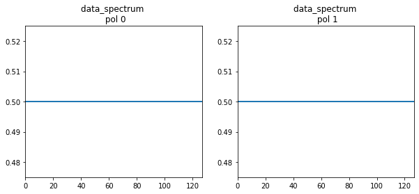
print('Data plots. Only point source:')
plot_ms_data(ms_name, 'data_spectrum')
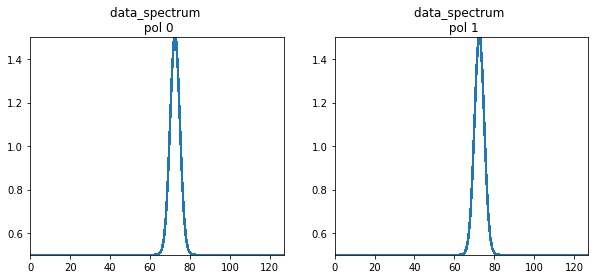
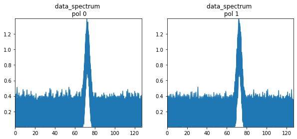
add_spectral_line(ms_name, chan_range=[60,86])
if verbose:
print('Data plots, + spectral line, width ~20% band:')
plot_ms_data(ms_name, 'data_spectrum')
# polynomial order 0,1,2,3 around 0.5Jy
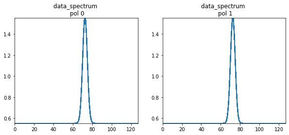
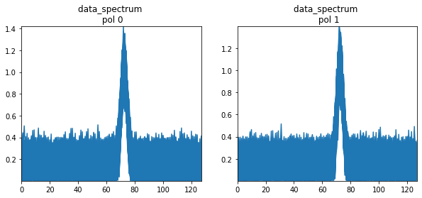
add_polynomial_cont(ms_name, pol_coeffs, spw_params['nchan'])
if verbose:
print('Data plots + polynomial cont:')
plot_ms_data(ms_name, 'data_spectrum')
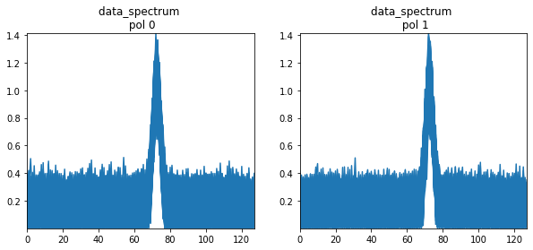
if noise_sigma:
add_ms_gaussian_noise(ms_name, noise_sigma)
if verbose:
print('Data plots + Gaussian noise:')
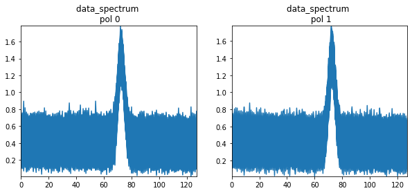
plot_ms_data(ms_name, 'data_spectrum')
Simple MS with continuum, line, and noise, plotted step by step
Using order 0 continuum.
The structure of this MS is the one used at the moment in the task test (test_task_req_uvcontsub). nchan=128. The spectral line is added to channels 60-85. The value of the fitspec parameter for this MS structure would be ‘0:0~59;86~127’
[34]:
os.system('rm -rf example_sim_alma_*.ms sim_alma_*.ms')
ms_name = 'example_sim_alma_noise_cont_poly_order_0.ms'
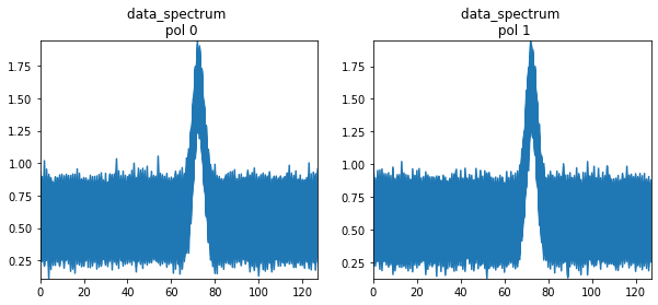
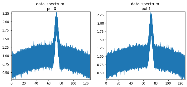
make_test_ms_alma_verif(ms_name, pol_coeffs=[0.05], verbose=True)
Data plots. Only point source:
/usr/local/lib/python3.7/dist-packages/ipykernel_launcher.py:62: UserWarning: Attempting to set identical bottom == top == 0.5 results in singular transformations; automatically expanding.
Data plots, + spectral line, width ~20% band:
Data plots + polynomial cont:
Data plots + Gaussian noise:
More simple examples of test MSs
[35]:
# Still make a trivial order 0 without noise, for the most basic verif test
ms_name = 'example_sim_alma_nonoise_cont_poly_order_0.ms'
make_test_ms_alma_verif(ms_name, pol_coeffs=[0.5], noise_sigma=None, verbose=False)
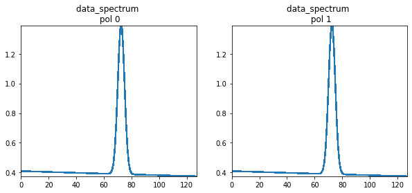
ms_name = 'example_sim_alma_nonoise_cont_poly_order_1.ms'
make_test_ms_alma_verif(ms_name, pol_coeffs=[-0.1, 0.75], noise_sigma=None, verbose=False)
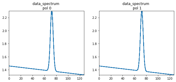
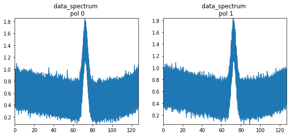
print('Plotting no-noise MS, with continuum as polynomial order 1')
plot_ms_data(ms_name, 'data_spectrum')
Plotting no-noise MS, with continuum as polynomial order 1
[36]:
!du -hsc *.ms
35M     example_sim_alma_noise_cont_poly_order_0.ms
35M     example_sim_alma_nonoise_cont_poly_order_0.ms
35M     example_sim_alma_nonoise_cont_poly_order_1.ms
12M     uvcont_noise_sub_0.ms
12M     uvcont_noise_sub_1.ms
12M     uvcont_noise_sub_2.ms
12M     uvcont_noise_sub_3.ms
12M     uvcont_nonoise_sub_1.ms
162M    total
[37]:
from casatasks import listobs
res = listobs(vis=ms_name)
import pprint
pprint.pprint(res)
print(res)
{'BeginTime': 59500.802114409686,
 'EndTime': 59500.80220700228,
 'IntegrationTime': 8.0,
 'field_0': {'code': '',
             'direction': {'m0': {'unit': 'rad', 'value': -1.0494882958398402},
                           'm1': {'unit': 'rad', 'value': 0.7109380541842404},
                           'refer': 'J2000',
                           'type': 'direction'},
             'name': 'simulated_source'},
 'nfields': 1,
 'numrecords': 3612,
 'scan_1': {'0': {'BeginTime': 59500.802114409686,
                  'EndTime': 59500.80220700228,
                  'FieldId': 0,
                  'FieldName': 'simulated_source',
                  'IntegrationTime': 2.0,
                  'SpwIds': array([0]),
                  'StateId': 0,
                  'nRow': 3612,
                  'scanId': 1}},
 'timeref': 'UTC'}
{'BeginTime': 59500.802114409686, 'EndTime': 59500.80220700228, 'IntegrationTime': 8.0, 'field_0': {'code': '', 'direction': {'m0': {'unit': 'rad', 'value': -1.0494882958398402}, 'm1': {'unit': 'rad', 'value': 0.7109380541842404}, 'refer': 'J2000', 'type': 'direction'}, 'name': 'simulated_source'}, 'nfields': 1, 'numrecords': 3612, 'scan_1': {'0': {'BeginTime': 59500.802114409686, 'EndTime': 59500.80220700228, 'FieldId': 0, 'FieldName': 'simulated_source', 'IntegrationTime': 2.0, 'SpwIds': array([0]), 'StateId': 0, 'nRow': 3612, 'scanId': 1}}, 'timeref': 'UTC'}
MeasurementSets with continuum polynomials of order 0, 1, 2, 3, etc.
[38]:
# Giving coefficients as [0.1, 0.45] == 0.1x + 0.45
polynomials = {0: [0.025],
1: [-0.1, 0.75],
2: [-1, 1, 0.15],
3: [1, -0.75, -0.25, 0.15]
# Order 3 could also be of the style (not sure what type we'd
# want):
# [-1.35, 0, 1.5, 0.2]
}
for order, poly in polynomials.items():
ms_name = f'sim_alma_cont_poly_order_{order}_nonoise.ms'
os.system('rm -rf sim_*.cl')
make_test_ms_alma_verif(ms_name, pol_coeffs=poly, noise_sigma=None, verbose=False)
ms_name = f'sim_alma_cont_poly_order_{order}_noise.ms'
os.system('rm -rf sim_*.cl')
make_test_ms_alma_verif(ms_name, pol_coeffs=poly, verbose=False)
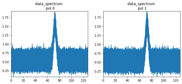
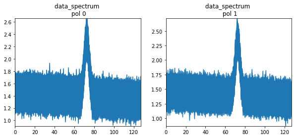
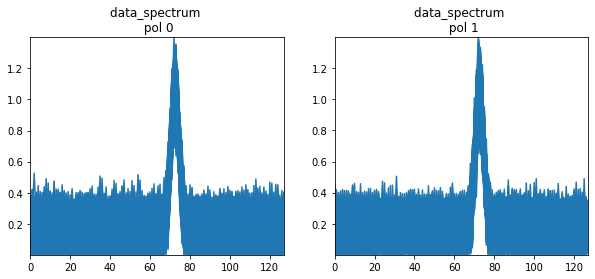
print(f'Plotting polynomial order {order}:')
plot_ms_data(ms_name, 'data_spectrum')
Plotting polynomial order 0:
Plotting polynomial order 1:
Plotting polynomial order 2:
Plotting polynomial order 3:
[39]:
# Check all MSs are there and their sizes
!du -hsc *.ms
35M     example_sim_alma_noise_cont_poly_order_0.ms
35M     example_sim_alma_nonoise_cont_poly_order_0.ms
35M     example_sim_alma_nonoise_cont_poly_order_1.ms
35M     sim_alma_cont_poly_order_0_noise.ms
35M     sim_alma_cont_poly_order_0_nonoise.ms
35M     sim_alma_cont_poly_order_1_noise.ms
35M     sim_alma_cont_poly_order_1_nonoise.ms
35M     sim_alma_cont_poly_order_2_noise.ms
35M     sim_alma_cont_poly_order_2_nonoise.ms
35M     sim_alma_cont_poly_order_3_noise.ms
35M     sim_alma_cont_poly_order_3_nonoise.ms
12M     uvcont_noise_sub_0.ms
12M     uvcont_noise_sub_1.ms
12M     uvcont_noise_sub_2.ms
12M     uvcont_noise_sub_3.ms
12M     uvcont_nonoise_sub_1.ms
440M    total
Noise level in the line free channels before and after continuum subtraction
When applying continuum subtraction, the output RMS increases with respect to the input RMS by a factor of
\(\mathrm{sqrt}(1+1/N_c)),\)
where \(N_c\) is the number of channels for which the continuum has been fitted. In the simple MeasurementSet examples above, where fitspec=’0:0~59;86~127’, \(N_c = 102\) (from the 128 channels, there are 60 (left) + 42 (right) line free channels and 26 line channels.
The output residual continuum flux deviates from 0 following a standard deviation of
\(N_l s (1 + N_l / N_c)\),
where \(N_l\) is the number of line channels (26 in the simple simulations above) and \(s\) is the sigma of the added artificial Gaussian noise.
Output RMS
Since a fit can never be noise free the output will always have more noise, although for a good fit this extra noise would probably be close to negligible when the number of channels to fit is sufficiently large.
In the case in which the simulation is a flat continuum (polynomial of order 0) with known artificial Gaussian noise of sigma \(s\), fitting a 0-order polynomial is numerically equivalent to compute the average across all the \(N_c\) channels (\(x_c\)). The standard error of that average is then \(s/\sqrt{N_c}\) and the variance \(s^2/N_c\). For a given visibility value in a channel (\(x_i\)), the value with continuum subtracted (\(x_i - x_c\)) has a variance of
\(var(x_i) + var(x_{mean}) = s^2 + s^2/N_c = s^2 (1+1/N_c)\).
In other words, the variance of the output has been increased by a factor (\(1+1/N_c)\) (or the RMS by a factor of \(\sqrt{1+1/N_c}\)). For the simulations above, where \(N_c = 102\) line-free channels than means a factor \(~1.005\). Note that this factor depends only on the number of line-free channels and is independent of the absolute values of the visibilities or the added noise.
Output residual continuum flux
Assuming a simulated line profile \(P_i\) with and additional continuum with a Gaussian distribution of mean \(C\) and sigma \(s\), each channel in the input spectrum is a statistical variable with a mean of \(P_i + C\) and a standard deviation of \(s\). Or in statistical notation:
\(x_i \sim N(P_i + C, s),\)
where \(N(m,s)\) denotes the normal distribution with mean \(m\) and sigma \(s\).
The integrated flux (\(F\)) computed on the output spectrum is the sum over \(N_l\) channels and is also a statistical variable that is the sum of several \(x_i\) minus the estimated continuum \(x_c\) that is itself a statistical variable:
\(x_c \sim N(C, \sqrt{(s^2/N_c})\)
\(F \sim N(\sum P_i + (N_l C -N_l C), \sqrt{N_l s^2 + N_l s^2 / N_c} ),\)
where \(\sum P_i\) is the summation of the profile over the \(N_l\) channels of the line.
The integrated flux minus the theoretical flux (\(\sum P_i\)) is also a statistical variable:
\(F - F_{theor} \sim N(0, \sqrt{N_l s^2 + N_l s^2 / N_c} ).\)
Or in other words: the measured flux in the output spectrum minus the theoretical flux follows a normal distribution that will have a mean of 0 and a standard deviation of \(\sqrt{N_l s^2 + N_l s^2 / N_c}\), or a variance of \(N_l s (1 + N_l / N_c)\).
The interesting point is that, for this model, the residual continuum flux is independent of the line flux, and it will deviate from 0 following a standard deviation of \(N_l s (1 + N_l / N_c)\).
Note that the analysis would be different if one assumes different models in which the flux of the line contributes to the noise, like a Poisson distribution. In this model it is assumed that the noise is constant and independent of the visibility value.
Continuum subtraction with uvcontsub
Several example commands to illustrate how uvcontsub is applied to the simulated MSs.
Using MeasurementSets for task verification test
[45]:
# Copy files to drive if needed to work with them outside of colab
copy_files = False
if 'google.colab' in str(get_ipython()) and copy_files:
  from google.colab import drive
  #drive.mount('/content/drive')
  !cp -r sim_*.ms /content/drive/MyDrive/sim_ms
[46]:
try:
from casatasks import uvcontsub
fitspec='0:0~59;86~127'
ms_uvcont = 'uvcont_noise_sub_0.ms'
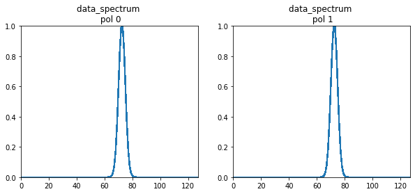
res = uvcontsub(vis='sim_alma_cont_poly_order_0_noise.ms', outputvis=ms_uvcont,
fitorder=0, fitspec=fitspec)
print(res)
print('uv-cont result, polynomial order 0')
plot_ms_data(ms_uvcont, 'data_spectrum')
ms_uvcont = 'uvcont_nonoise_sub_1.ms'
res = uvcontsub(vis='sim_alma_cont_poly_order_1_nonoise.ms', outputvis=ms_uvcont,
fitorder=1, fitspec=fitspec)
print('uv-cont result (no noise), polynomial order 1')
plot_ms_data(ms_uvcont, 'data_spectrum')
ms_uvcont = 'uvcont_noise_sub_1.ms'
res = uvcontsub(vis='sim_alma_cont_poly_order_1_noise.ms', outputvis=ms_uvcont,
fitorder=1, fitspec=fitspec)
print('uv-cont result, polynomial order 1')
plot_ms_data(ms_uvcont, 'data_spectrum')
ms_uvcont = 'uvcont_noise_sub_2.ms'
res = uvcontsub(vis='sim_alma_cont_poly_order_2_noise.ms', outputvis=ms_uvcont,
fitorder=2, fitspec=fitspec)
print('uv-cont result, polynomial order 2')
plot_ms_data(ms_uvcont, 'data_spectrum')
ms_uvcont = 'uvcont_noise_sub_3.ms'
res = uvcontsub(vis='sim_alma_cont_poly_order_3_noise.ms', outputvis=ms_uvcont,
fitorder=3, fitspec=fitspec)
print('uv-cont result, polynomial order 3')
plot_ms_data(ms_uvcont, 'data_spectrum')
except ImportError as exc:
print('Import error, most likely related to casatasks/tools not yet including '
f'new uvcontsub: {exc}')
{'description': 'summary of data fitting results in uv-continuum subtraction', 'goodness_of_fit': {'field': {'0': {'scan': {'1': {'spw': {'0': {'polarization': {'0': {'chi_squared': {'average': {'imag': 1.0526342391967773, 'real': 0.9639652371406555}, 'max': {'imag': 1.1145819425582886, 'real': 1.0763975381851196}, 'min': {'imag': 1.081458568572998, 'real': 0.7475039958953857}}, 'count': 4}, '1': {'chi_squared': {'average': {'imag': 1.047758936882019, 'real': 1.035971760749817}, 'max': {'imag': 1.0653717517852783, 'real': 1.148736834526062}, 'min': {'imag': 0.9923614263534546, 'real': 0.9539858102798462}}, 'count': 4}}}}}}}}}}
uv-cont result, polynomial order 0
uv-cont result (no noise), polynomial order 1
uv-cont result, polynomial order 1
uv-cont result, polynomial order 2
uv-cont result, polynomial order 3
Produce simulated MeasurementSets - for further testing and characterization
As opposed to the MSs produced for the task verification test, in the following functions we produce MSs without adding polynomials to the real and imaginary part of the visibilities. These MSs can be used to test the behavior of the task with sources
[47]:
def make_test_ms_alma_further(ms_name, noise_sigma='0.5Jy', verbose=True):
  """
  Adds a point source, a spectral line, noise

  Args:
      noise_sigma: sigma for the Gaussian noise, set to None for no noise
      verbose: print and plot what is being done
  """
  ant_config = 'alma.cycle8.8.cfg'
  spw_params = {'name': "Simulated_Band",
                'freq': '150GHz',
                'nchan': 128}

  make_ms_frame(ms_name, ant_config=ant_config, spw_params=spw_params)

  add_point_source_component(ms_name, freq='125GHz', flux=0.5,
                             spectrumtype='spectral index', index=-1.1)

  if verbose:
    print('Data plots. Only point source:')
    plot_ms_data(ms_name, 'data_spectrum')

  add_spectral_line(ms_name, chan_range=[60,86])
  if verbose:
    print('Data plots, + spectral line, width ~20% band:')
    plot_ms_data(ms_name, 'data_spectrum')

  if noise_sigma:
    add_ms_gaussian_noise(ms_name, noise_sigma)
    if verbose:
      print('Data plots + Gaussian noise:')
      plot_ms_data(ms_name, 'data_spectrum')
Simple MSs
[48]:
ms_name = 'sim_alma_source_phase_center_nonoise.ms'
make_test_ms_alma_further(ms_name, noise_sigma=None, verbose=False)
print('Plotting no-noise MS, with spectral index source')
plot_ms_data(ms_name, 'data_spectrum')

ms_name = 'sim_alma_source_phase_center_noise.ms'
make_test_ms_alma_further(ms_name, noise_sigma='0.1Jy', verbose=False)
print('Plotting no-noise MS, with spectral index source')
plot_ms_data(ms_name, 'data_spectrum')
Plotting no-noise MS, with spectral index source
Plotting no-noise MS, with spectral index source