Open in Colab: https://colab.research.google.com/github/casangi/casadocs/blob/20cf5f0/docs/notebooks/image_combination.ipynb
Image Combination
Joint Single Dish and Interferometer Image Reconstruction
The SDINT imaging algorithm allows joint reconstruction of wideband single dish and interferometer data. This algorithm is available in the task sdintimaging and described in Rau, Naik & Braun (2019).
Experience with joint reconstruction of wideband single dish and interferometer data in CASA using the sdintimaging task is limited. Only part of the parameter space has been validated. The usage modes that have been tested are documented below.
SDINT Algorithm
Interferometer data are gridded into an image cube (and corresponding PSF). The single dish image and PSF cubes are combined with the interferometer cubes in a feathering step. The joint image and PSF cubes then form inputs to any deconvolution algorithm (in either cube or mfs/mtmfs modes). Model images from the deconvolution algorithm are translated back to model image cubes prior to subtraction from both the single dish image cube as well as the interferometer data to form a new pair of residual image cubes to be feathered in the next iteration. In the case of mosaic imaging, primary beam corrections are performed per channel of the image cube, followed by a multiplication by a common primary beam, prior to deconvolution. Therefore, for mosaic imaging, this task always implements conjbeams=True and normtype=’flatnoise’.
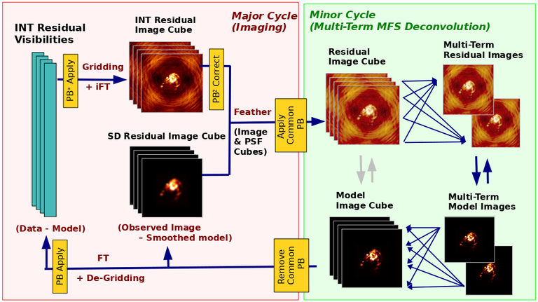
The input single dish data are the single dish image and psf cubes. The input interferometer data is a MeasurementSet. In addition to imaging and deconvolution parameters from interferometric imaging (task tclean), there are controls for a feathering step to combine interferometer and single dish cubes within the imaging iterations. Note that the above diagram shows only the ‘mtmfs’ variant. Cube deconvolution proceeds directly with the cubes in the green box above, without the extra conversion back and forth to the multi-term basis. Primary beam handling is also not shown in this diagram, but full details (via pseudocode) are available in the reference publication.
The parameters used for controlling the joint deconvolution are described on the sdintimaging task pages.
Usage Modes
The task sdintimaging contains the algorithm for joint reconstruction of wideband single dish and interferometer data. The sdintimaging task shares a significant number of parameters with the tclean task, but also contains unique parameters. A detailed overview of these parameters, and how to use them, can be found in the CASA Docs task pages of sdintimaging.
As seen from the diagram above and described on the sdintimaging task pages, there is considerable flexibility in usage modes. One can choose between interferometer-only, singledish-only and joint interferometer-singledish imaging. Only the latter constitutes actual data combination. The other two are more useful for testing. Outputs in all three cases are restored images and associated data products (similar to task tclean).
The following usage modes are available in the (experimental) sdintimaging task. Tested modes include all 12 combinations of:
Cube Imaging : All combinations of the following options.
specmode = ‘cube’
deconvolver = ‘multiscale’, ‘hogbom’
usedata = ‘sdint’, ‘sd’ , ‘int’
gridder = ‘standard’, ‘mosaic’
parallel = False, True
Wideband Multi-Term Imaging : All combinations of the following options.
specmode = ‘mfs’
deconvolver = ‘mtmfs’ ( nterms=1 for a single-term MFS image, and nterms>1 for multi-term MFS image. Tests use nterms=2 )
usedata = ‘sdint’, ‘sd’ , ‘int’
gridder = ‘standard’, ‘mosaic’
parallel = False, True
NOTE: Currently only stokes=”I” is supported when usedata=”sdint”
NOTE: When the INT and/or SD cubes have flagged (and therefore empty) channels, only those channels that have non-zero images in both the INT and SD cubes are used for the joint reconstruction.
NOTE: Single-plane joint imaging presently only works with deconvolver=’mtmfs’ and nterms=1.
NOTE: All other modes allowed by the new sdintimaging task are currently untested. Tests will be added in subsequent releases.
Examples/Demos
Basic test results
The sdintimaging task was run on a pair of simulated test datasets. Both contain a flat spectrum extended emission feature plus three point sources, two of which have spectral index=-1.0 and one which is flat-spectrum (rightmost point). The scale of the top half of the extended structure was chosen to lie within the central hole in the spatial-frequency plane at the middle frequency of the band so as to generate a situation where the interferometer-only imaging is difficult.
Please refer to the publication for a more detailed analysis of the imaging quality and comparisons of images without and with SD data. Another study of interest is Plunkett, Hacar, Moser-Fischer et al. 2023 which compares the performance of sdintimaging with several other data combination methods.
Images from a run on the ALMA M100 12m+7m+TP Science Verification Data suite are also shown below.
Single Pointing Simulation :
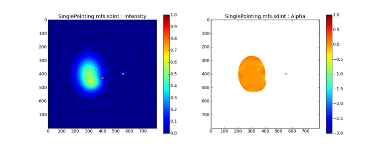
Wideband Multi-Term Imaging ( deconvolver=’mtmfs’, specmode=’mfs’ )
SD + INT
A joint reconstruction accurately reconstructs both intensity and spectral index for the extended emission as well as the compact sources.
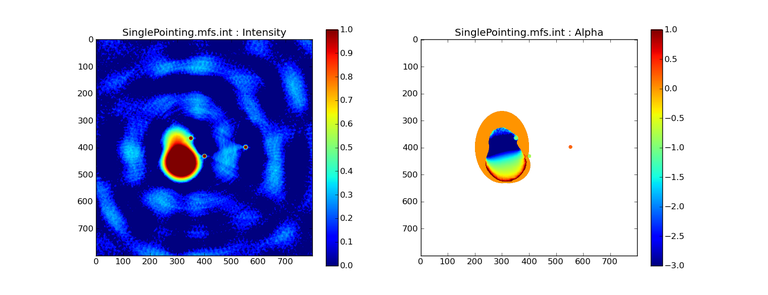
INT-only
The intensity has negative bowls and the spectral index is overly steep, especially for the top half of the extended component.
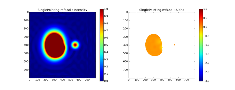
SD-only
The spectral index of the extended emission is accurate (at 0.0) and the point sources are barely visible at this SD angular resolution.
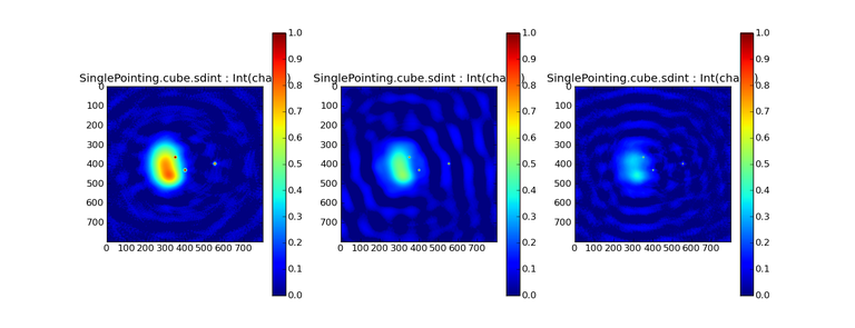
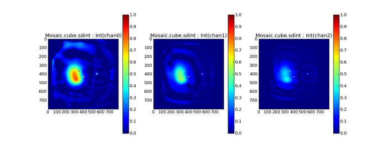
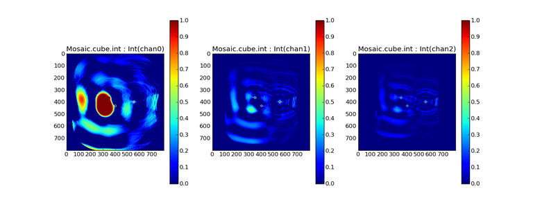
Cube Imaging ( deconvolver=’multiscale’, specmode=’cube’ )
SD + INT
A joint reconstruction has lower artifacts and more accurate intensities in all three channels, compared to the int-only reconstructions below
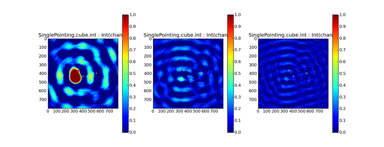
INT-only
The intensity has negative bowls in the lower frequency channels and the extended emission is largely absent at the higher frequencies.
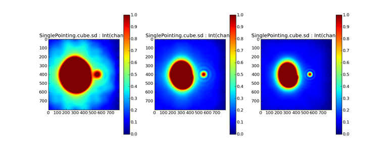
SD-only
A demonstration of single-dish cube imaging with deconvolution of the SD-PSF.
In this example, iterations have not been run until full convergence, which is why the sources still contain signatures of the PSF.
Mosaic Simulation
An observation of the same sky brightness was simulated with 25 pointings.
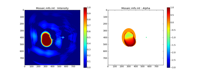
Wideband Multi-Term Mosaic Imaging ( deconvolver=’mtmfs’, specmode=’mfs’ , gridder=’mosaic’ )
SD + INT
A joint reconstruction accurately reconstructs both intensity and spectral index for the extended emission as well as the compact sources.
This is a demonstration of joint mosaicing along with wideband single-dish and interferometer combination.

INT-only
The intensity has negative bowls and the spectral index is strongly inaccurate. Note that the errors are slightly less than the situation with the single-pointing example (where there was only one pointing’s worth of uv-coverage).
Cube Mosaic Imaging ( deconvolver=’multiscale’, specmode=’cube’, gridder=’mosaic’ )
SD + INT
A joint reconstruction produces better per-channel reconstructions compared to the INT-only situation shown below.
This is a demonstration of cube mosaic imaging along with SD+INT joint reconstruction.
INT-only
Cube mosaic imaging with only interferometer data. This clearly shows negative bowls and artifacts arising from the missing flux.
ALMA M100 Spectral Cube Imaging : 12m + 7m + TP
The sdintimaging task was run on the ALMA M100 Science Verification Datasets.
The single dish (TP) cube was pre-processed by adding per-plane restoringbeam information.
Cube specification parameters were obtained from the SD Image as follows
from sdint_helper import *
sdintlib = SDINT_helper()
sdintlib.setup_cube_params(sdcube='M100_TmP')

Output : Shape of SD cube : [90 90  1 70\]
Coordinate ordering : ['Direction', 'Direction', 'Stokes', 'Spectral']
nchan = 70
start = 114732899312.0Hz
width = -1922516.74324Hz
Found 70 per-plane restoring beams\#

(For specmode='mfs' in sdintimaging, please remember to set 'reffreq' to a value within the freq range of the cube.

Returned Dict : {'nchan': 70, 'start': '114732899312.0Hz', 'width': '-1922516.74324Hz'}
Task sdintimaging was run with automatic SD-PSF generation, n-sigma stopping thresholds, a pb-based mask at the 0.3 gain level, and no other deconvolution masks (interactive=False).
sdintimaging(usedata="sdint", sdimage="../M100_TP", sdpsf="",sdgain=3.0,
             dishdia=12.0, vis="../M100_12m_7m", imagename="try_sdint_niter5k",
             imsize=1000, cell="0.5arcsec", phasecenter="J2000 12h22m54.936s +15d48m51.848s",
             stokes="I", specmode="cube", reffreq="", nchan=70, start="114732899312.0Hz",
             width="-1922516.74324Hz", outframe="LSRK", veltype="radio",
             restfreq="115.271201800GHz", interpolation="linear",
             perchanweightdensity=True, gridder="mosaic", mosweight=True,
             pblimit=0.2, deconvolver="multiscale", scales=[0, 5, 10, 15, 20],
             smallscalebias=0.0, pbcor=False, weighting="briggs", robust=0.5,
             niter=5000, gain=0.1, threshold=0.0, nsigma=3.0, interactive=False,
             usemask="user", mask="", pbmask=0.3)
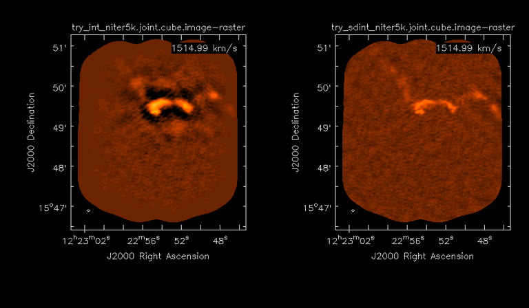
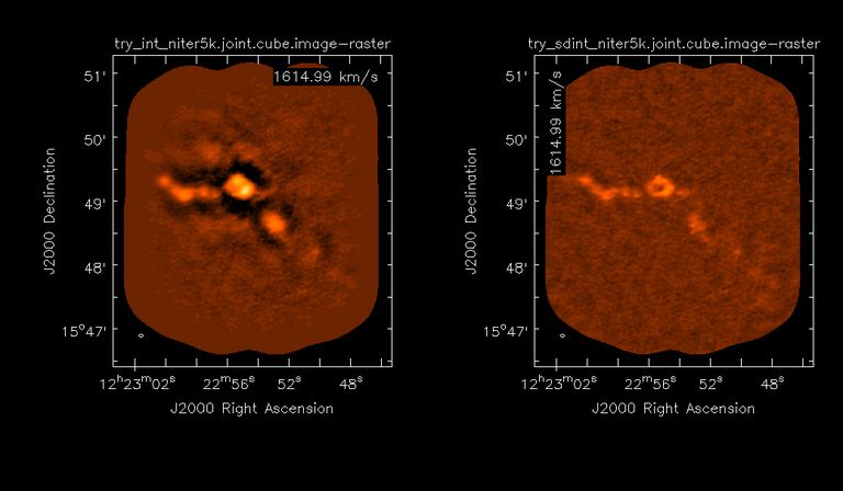
Results from two channels are show below.
LEFT : INT only (12m+7m) and RIGHT : SD+INT (12m + 7m + TP)
Channel 23
Channel 43
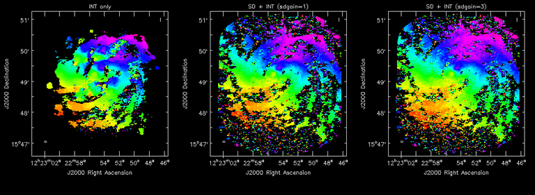
Moment 0 Maps : LEFT : INT only. MIDDLE : SD + INT with sdgain=1.0 RIGHT : SD + INT with sdgain=3.0

Moment 1 Maps : LEFT : INT only. MIDDLE : SD + INT with sdgain=1.0 RIGHT : SD + INT with sdgain=3.0
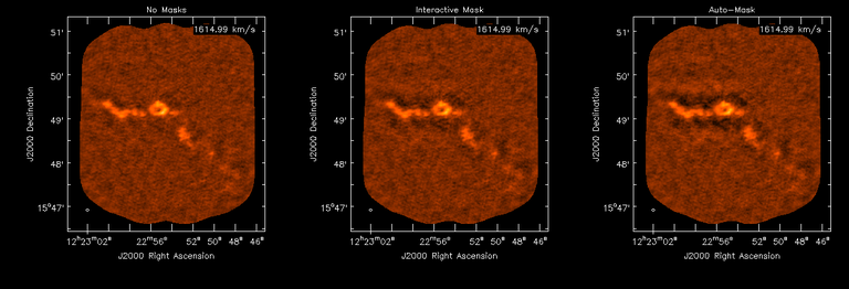
A comparison (shown for one channel) with and without masking is shown below.
Notes :
In the reconstructed cubes, negative bowls have clearly been eliminated by using sdintimaging to combine interferometry + SD data. Residual images are close to noise-like too (not pictured above) suggesting a well-constrained and steadily converging imaging run.
The source structure is visibly different from the INT-only case, with high and low resolution structure appearing more well defined. However, the high-resolution peak flux in the SDINT image cube is almost a factor of 3 lower than the INT-only. While this may simply be because of deconvolution uncertainty in the ill-constrained INT-only reconstruction, it requires more investigation to evaluate absolute flux correctness. For example, it will be useful to evaluate if the INT-only reconstructed flux changes significantly with careful hand-masking.
Compare with a Feathered image : http://www.astroexplorer.org/details/apjaa60c2f1 : The reconstructed structure is consistent.
The middle and right panels compare reconstructions with different values of sdgain (1.0 and 3.0). The sdgain=3.0 run has a noticeable emphasis on the SD flux in the reconstructed moment maps, while the high resolution structures have the same are the same between sdgain=1 and 3. This is consistent with expectations from the algorithm, but requires further investigation to evaluate robustness in general.
Except for the last panel, no deconvolution masks were used (apart from a pbmask at the 0.3 gain level). The deconvolution quality even without masking is consistent with the expectation that when supplied with better data constraints in a joint reconstruction, the native algorithms are capable of converging on their own. In this example (same niter and sdgain), iterative cleaning with interactive and auto-masks (based mostly on interferometric peaks in the images) resulted in more artifacts compared to a run that allowed multi-scale clean to proceed on its own.
The results using sdintimaging on these ALMA data can be compared with performance results when using feather, and when using tp2vis (ALMA study by J. Koda and P. Teuben).
Fitting a new restoring beam to the Feathered PSF
Since the deconvolution uses a joint SD+INT point spread function, the restoring beam is re-fitted after the feather step within the sdintimaging task. As a convenience feature, the corresponding tool method is also available to the user and may be used to invoke PSF refitting standalone, without needing an MS or any gridding of weights to make the PSF. This method will look for the imagename.psf (or imagename.psf.tt0), fit and set the new restoring beam. It is tied to the naming convention of tclean.
synu = casac.synthesisutils();
synu.fitPsfBeam(imagename='qq', psfcutoff=0.3) # Cubes
synu.fitPsfBeam(imagename='qq', nterms=2, psfcutoff=0.3) # Multi-term
Tested Use Cases
The following is a list of use cases that have simulation-based functional verification tests within CASA.
Wideband mulit-term imaging (SD+Int)
Wideband data single field imaging by joint-reconstruction from single dish and interferometric data to obtain the high resolution of the interferometer while account for the zero spacing information. Use multi-term multi-frequency synthesis (MTMFS) algorithm to properly account for spectral information of the source.
Wideband multi-term imaging: Int only
The same as #1 except for using interferometric data only, which is useful to make a comparison with #1 (i.e. effect of missing flux). This is equivalent to running ‘mtmfs’ with specmode=’mfs’ and gridder=’standard’ in tclean
Wideband multi-term imaging: SD only
The same as #1 expect for using single dish data only which is useful to make a comparison with #1 (i.e. to see how much high resolution information is missing). Also, sometimes, the SD PSF has significant sidelobes (Airy disk) and even single dish images can benefit from deconvolution. This is a use case where wideband multi-term imaging is applied to SD data alone to make images at the highest possible resolution as well as to derive spectral index information.
Single field cube imaging: SD+Int
Spectral cube single field imaging by joint reconstruction of single dish and interferometric data to obtain single field spectral cube image.
Use multi-scale clean for deconvolution
Single field cube imaging: Int only
The same as #4 except for using the interferometric data only, which is useful to make a comparison with #4 (i.e. effect of missing flux). This is equivalent to running ‘multiscale’ with specmode=’cube’ and gridder=’standard’ in tclean.
Single field cube imaging: SD only
The same as #4 except for using the single dish data only, which is useful to make a comparison with #4
(i.e. to see how much high resolution information is missing)
Also, it addresses the use case where SD PSF sidelobes are significant and where the SD images could benefit from multiscale (or point source) deconvolution per channel.
Wideband multi-term mosaic Imaging: SD+Int
Wideband data mosaic imaging by joint-reconstruction from single dish and interferometric data to obtain the high resolution of the interferometer while account for the zero spacing information.
Use multi-term multi-frequency synthesis (MTMFS) algorithm to properly account for spectral information of the source. Implement the concept of conjbeams (i.e. frequency dependent primary beam correction) for wideband mosaicing.
Wideband multi-term mosaic imaging: Int only
The same as #7 except for using interferometric data only, which is useful to make a comparison with #7 (i.e. effect of missing flux). Also, this is an alternate implementation of the concept of conjbeams ( frequency dependent primary beam correction) available via tclean, and which is likely to be more robust to uv-coverage variations (and sumwt) across frequency.
Wideband multi-term mosaic imaging: SD only
The same as #7 expect for using single dish data only which is useful to make a comparison with #7 (i.e. to see how much high resolution information is missing). This is the same situation as (3), but made on an image coordinate system that matches an interferometer mosaic mtmfs image.
Cube mosaic imaging: SD+Int
Spectral cube mosaic imaging by joint reconstruction of single dish and interferometric data. Use multi-scale clean for deconvolution.
Cube mosaic imaging: Int only
The same as #10 except for using the intererometric data only, which is useful to make a comparison with #10 (i.e. effect of missing flux). This is the same use case as gridder=’mosaic’ and deconvolver=’multiscale’ in tclean for specmode=’cube’.
Cube mosaic imaging: SD only
The same as #10 except for using the single dish data only, which is useful to make a comparison with #10 (i.e. to see how much high resolution information is missing). This is the same situation as (6), but made on an image coordinate system that matches an interferometer mosaic cube image.
Wideband MTMFS SD+INT with channel 2 flagged in INT
The same as #1, but with partially flagged data in the cubes. This is a practical reality with real data where the INT and SD data are likely to have gaps in the data due to radio frequency interferenece or other weight variations.
Cube SD+INT with channel 2 flagged
The same as #4, but with partially flagged data in the cubes. This is a practical reality with real data where the INT and SD data are likely to have gaps in the data due to radio frequency interferenece or other weight variations.
Wideband MTMFS SD+INT with sdpsf=””
The same as #1, but with an unspecified sdpsf. This triggers the auto-calculation of the SD PSF cube using restoring beam information from the regridded input sdimage.
INT-only cube comparison between tclean and sdintimaging
Compare cube imaging results for a functionally equivalent run.
INT-only mtmfs comparison between tclean and sdintimaging
Compare mtmfs imaging results for a functionally equivalent run. Note that the sdintimaging task implements wideband primary beam correction in the image domain on the cube residual image, whereas tclean uses the ‘conjbeams’ parameter to apply an approximation of this correction during the gridding step.
Note : Serial and Parallel Runs for an ALMA test dataset have been shown to be consistent to a 1e+6 dynamic range, consistent with differences measured for our current implementation of cube parallelization.
References
Urvashi Rau, Nikhil Naik, and Timothy Braun 2019 AJ 158, 1
https://github.com/urvashirau/WidebandSDINT
Feather & CASAfeather
Feathering is a technique used to combine a Single Dish (SD) image with an interferometric image of the same field.The goal of this process is to reconstruct the source emission on all spatial scales, ranging from the small spatial scales measured by the interferometer to the large-scale structure measured by the single dish. To do this, feather combines the images in Fourier space, weighting them by the spatial frequency response of each image. This technique assumes that the spatial frequencies of the single dish and interferometric data partially overlap. The subject of interferometric and single dish data combination has a long history. See the introduction of Koda et al 2011 (and references therein) [1] for a concise review, and Vogel et al 1984 [2], Stanimirovic et al 1999 [3], Stanimirovic 2002 [4], Helfer et al 2003 [5], and Weiss et al 2001 [6], among other referenced papers, for other methods and discussions concerning the combination of single dish and interferometric data.
The feathering algorithm implemented in CASA is as follows:
Regrid the single dish image to match the coordinate system, image shape, and pixel size of the high resolution image.
Transform each image onto uniformly gridded spatial-frequency axes.
Scale the Fourier-transformed low-resolution image by the ratio of the volumes of the two ‘clean beams’ (high-res/low-res) to convert the single dish intensity (in Jy/beam) to that corresponding to the high resolution intensity (in Jy/beam). The volume of the beam is calculated as the volume under a two dimensional Gaussian with peak 1 and major and minor axes of the beam corresponding to the major and minor axes of the Gaussian.
Add the Fourier-transformed data from the high-resolution image, scaled by \((1-wt)\) where \(wt\) is the Fourier transform of the ‘clean beam’ defined in the low-resolution image, to the scaled low resolution image from step 3.5. Transform back to the image plane.
The input images for feather must have the following characteristics:
Both input images must have a well-defined beam shape for this task to work, which will be a ‘clean beam’ for interferometric images and a ‘primary-beam’ for a single-dish image. The beam for each image should be specified in the image header. If a beam is not defined in the header or feather cannot guess the beam based on the telescope parameter in the header, then you will need to add the beam size to the header using imhead.
Both input images must have the same flux density normalization scale. If necessary, the SD image should be converted from temperature units to Jy/beam. Since measuring absolute flux levels is difficult with single dishes, the single dish data is likely to be the one with the most uncertain flux calibration. The SD image flux can be scaled using the parameter sdfactor to place it on the same scale as the interferometer data. The casafeather task (see below) can be used to investigate the relative flux scales of the images.
Feather attemps to regrid the single dish image to the interferometric image. Given that the single dish image frequently originates from other data reduction packages, CASA may have trouble performing the necessary regridding steps. If that happens, one may try to regrid the single dish image manually to the interferometric image. CASA has a few tasks to perform individual steps, including imregrid for coordinate transformations, imtrans to swap and reverse coordinate axes, the tool ia.adddegaxes() for adding degenerate axes (e.g. a single Stokes axis). See the “Image Analysis” chapter for additional options. If you have trouble changing image projections, you can try the montage package, which also has an associated python wrapper.
If you are feathering large images together, set the numbers of pixels along the X and Y axes to composite (non-prime) numbers in order to improve the algorithm speed. In general, FFTs work much faster on even and composite numbers. Then use the subimage task or tool to trim the number of pixels to something desirable.
Inputs for task feather
The inputs for feather are:
#feather :: Combine two images using their Fourier transforms
imagename       = ''     #Name of output feathered image
highres         = ''     #Name of high resolution (interferometer) image
lowres          = ''     #Name of low resolution (single dish) image
sdfactor        = 1.0    #Scale factor to apply to Single Dish image
effdishdiam     = -1.0   #New effective SingleDish diameter to use in m
lowpassfiltersd = False  #Filter out the high spatial frequencies of the SD image
The SD data cube is specified by the lowres parameter and the interferometric data cube by the highres parameter. The combined, feathered output cube name is given by the imagename parameter. The parameter sdfactor can be used to scale the flux calibration of the SD cube. The parameter effdishdiam can be used to change the weighting of the single dish image.
The weighting functions for the data are usually the Fourier transform of the Single Dish beam FFT(PBSD) for the Single dish data, and the inverse, 1-FFT(PBSD), for the interferometric data. It is possible, however, to change the weighting functions by pretending that the SD is smaller in size via the effdishdiam parameter. This tapers the high spatial frequencies of the SD data and adds more weight to the interferometric data. The lowpassfiltersd can take out non-physical artifacts at very high spatial frequencies that are often present in SD data.
Note that the only inputs are for images; feather will attempt to regrid the images to a common shape, i.e. pixel size, pixel numbers, and spectral channels. If you are having issues with the regridding inside feather, you may consider regridding using the imregrid and specsmooth tasks.
The feather task does not perform any deconvolution but combines the single dish image with a presumably deconvolved interferometric image. The short spacings of the interferometric image that are extrapolated by the deconvolution process will be those that are down-weighted the most when combined with the single dish data. The single dish image must have a well-defined beam shape and the correct flux units for a model image (Jy/beam instead of Jy/pixel). Use the tasks imhead and immath first to convert if needed.
Starting with a cleaned synthesis image and a low resolution image from a single dish telescope, the following example shows how they can be feathered:
feather(imagename ='feather.im',       #Create an image called feather.im
        highres   ='synth.im',         #The synthesis image is called synth.im
        lowres    ='single_dish.im')   #The SD image is called single_dish.im
Visual Interface for feather (casafeather)
CASA also provides a visual interface to the feather task. The interface is run from a command line outside CASA by typing casafeather in a shell. An example of the interface is shown below. To start, one needs to specify a high and a low resolution image, typically an interferometric and a single dish map. Note that the single dish map needs to be in units of Jy/beam. The output image name can be specified. The non-deconvolved (dirty) interferometric image can also be specified to use as diagnostic of the relative flux scaling of the single dish and interferometer images. See below for more details. At the top of the display, the parameters effdshdiameter and sdfactor can be provided in the “Effective Dish Diameter” and “Low Resolution Scale Factor” input boxes. One you have specified the images and parameters, press the “Feather” button in the center of the GUI window to start the feathering process. The feathering process here includes regridding the low resolution image to the high resolution image.
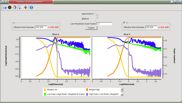
Figure 1: The panel shows the “Original Data Slice”, which are cuts through the u and v directions of the Fourier-transformed input images. Green is the single dish data (low resolution) and purple the interferometric data (high resolution). To bring them on the same flux scale, the low data were convolved to the high resolution beam and vice versa (selectable in color preferences). In addition, a single dish scaling of 1.2 was applied to adjust calibration differences. The weight functions are shown in yellow (for the low resolution data) and orange (for the high resolution data). The weighting functions were also applied to the green and purple slices. Image slices of the combined, feathered output image are shown in blue. The displays also show the location of the effective dish diameter by the vertical line. This value is kept at the original single dish diameter that is taken from the respective image header.
The initial casafeather display shows two rows of plots. The panel shows the “Original Data Slice”, which are either cuts through the u and v directions of the Fourier-transformed input images or a radial average. A vertical line shows the location of the effective dish diameter(s). The blue lines are the combined, feathered slices.
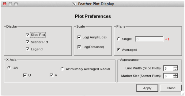
Figure 2: The casafeather “customize” window.
The ‘Customize’ button (gear icon on the top menu page) allows one to set the display parameters. Options are to show the slice plot, the scatter plot, or the legend. One can also select between logarithmic and linear axes; a good option is usually to make both axes logarithmic. You can also select whether the x-axis for the slices are in the u, or v, or both directions, or, alternatively a radial average in the uv-plane. For data cubes, one can also select a particular velocity plane, or to average the data across all velocity channels. The scatter plot can display any two data sets on the two axes, selected from the ‘Color Preferences’ menu. The data can be the unmodified, original data, or data that have been convolved with the high or low resolution beams. One can also select to display data that were weighted and scaled by the functions discussed above.
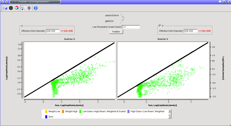
Figure 3: The scatter plot in casafeather. The low data, convolved with high beam, weighted and scaled is still somewhat below the equality line (plotted against high data, convolved with low beam, weighted). In this case one can try to adjust the “low resolution scale factor” to bring the values closer to the line of equality, ie. to adjust the calibration scales.
Plotting the data as a scatter plot is a useful diagnostic tool for checking for differences in flux scaling between the high and low resolution data sets.The dirty interferometer image contains the actual flux measurements made by the telescope. Therefore, if the single dish scaling is correct, the flux in the dirty image convolved with the low resolution beam and with the appropriate weighting applied should be the same as the flux of the low-resolution data convolved with the high resolution beam once weighted and scaled. If not, the sdfactor parameter can be adjusted until they are the same. One may also use the cleaned high resolution image instead of the dirty image, if the latter is not available. However, note that the cleaned high resolution image already contains extrapolations to larger spatial scales that may bias the comparison.
Bibliography
Koda et al 2011 (http://adsabs.harvard.edu/abs/2011ApJS..193…19K)
Vogel et al 1984 (http://adsabs.harvard.edu/abs/1984ApJ…283..655V)
Stanimirovic et al 1999 (http://adsabs.harvard.edu/abs/1999MNRAS.302..417S)
Stanimirovic et al 2002 (http://adsabs.harvard.edu/abs/2002ASPC..278..375S)
Helfer et al 2003 (http://adsabs.harvard.edu/abs/2003ApJS..145..259H)
Weiss et al 2001 (http://adsabs.harvard.edu/abs/2001A%26A…365..571W)
[ ]: